Lab 2
Scopes and Signals
Introduction
This lab assignment has three purposes:
-
Learn how to use an oscilloscope to observe and analyze signals.
-
Learn how to set up the oscilloscope triggering so both periodic and non-periodic signals can be clearly seen.
-
Use the oscilloscope to examine how long it takes for the input a system to affect the output.
Due to the number of students in the lab session there may not be sufficient oscilloscopes for each student to work individually. In this case you can work with a partner as a team of two. Teams of three should not be necessary and will only be allowed with the instructor’s approval. If you are working with a partner, everyone on the team should take turns working with the oscilloscope and doing the breadboard wiring so all team members learn how to do this. Don’t just sit there and watch someone else do the work. In future labs you will have to do the work all by yourself and this is your chance to learn how to do it.
Important: All students are required to submit their own copy of the Lab 2 answers by the due date even if you are working with a partner.
For a copy of the Lab 2 grading sheet, click here
Task 1: Learn to Use the Oscilloscope
An oscilloscope is used to show a graph of one or more signals as they change with time. The scope plots a picture of the signal showing the signal’s:
- Voltage level along the vertical axis, and
- Time along the horizontal axis
By displaying multiple signals on the same plot, it’s possible to see how they are interacting with each other. The scopes in VHE 205 are capable of displaying signals from four separate sources at the same time on the display. These are shown as channels 1 through 4 on the screen.
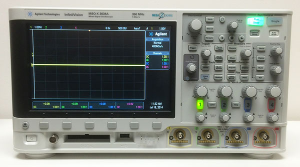
Note: The oscilloscopes in VHE 205 were made by Agilent, but the company is now called Keysight. Some of the pictures of the scope screens many show the Agilent name, while others may say Keysight, but the only difference is in the name. If the name on your scope screen doesn’t match the one in this web page, just ignore the mismatch.
To get started follow the steps below.
-
Turn on the oscilloscope by pressing the white button in the lower left of the front panel and wait for it to go through a bunch of self tests. In less than a minute it should be ready to go. If the scope doesn’t turn on, check that the power cord on the back is plugged into both the scope and an outlet below the bench.
-
Press the “Default Setup” button in the upper right portion of the front panel. This should restore the scope to the default settings in case someone has altered them.
-
After it says on the screen that the default setup has been restored, press the “Back” button in the lower left corner. You should see a screen like the one below. It may take two presses of “Back” to get to this screen.
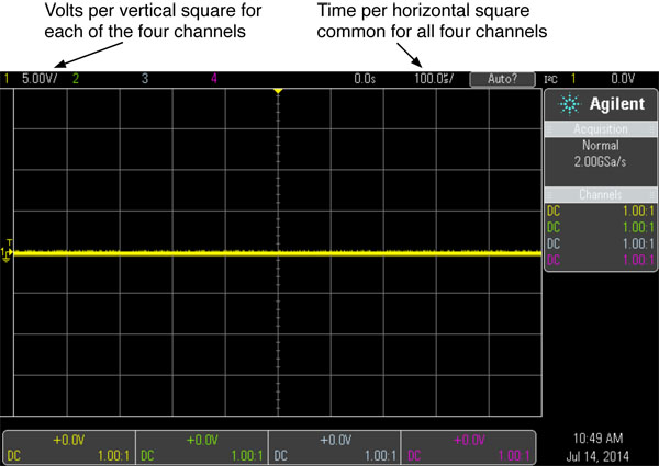
Notice the grid lines on the screen. There are eight vertical grid spaces (a.k.a. “divisions”) and ten horizontal “divisions”. These can be used in conjunction with the vertical and horizontal scale factors to measure the voltages and timing of signals. The first two numbers to look for are the scale factors for the vertical and horizontal axis. The vertical scale factor is shown in the upper left corner of the screen, and the horizontal scale factor is also along top about 2/3 of the way to the right side.
Note: Each of the four channels can have a different vertical scale factor and these are shown along the upper left of the screen. For example, channel 1 can be displayed with each division representing 1V while channel 2 is displayed 5V per division. In the default settings, only channel 1 (yellow) is turned on, and the display shows that the vertical scale factor is “5.00V”. This means that each of the grid lines represents 5 volts of signal level. The horizontal scale factor is set to “100μs” meaning that the signal is plotted with each horizontal grid space representing 100 microseconds of time. We’ll be using the grid lines and the vertical and horizontal scale factors to make voltage and time measurements on signals.
Since there is no input signal connected to channel 1, the plot or “trace” for channel 1 is just a horizontal line across the screen. Look at the left side of the screen where the horizontal line ends. You should see a small “Ground” symbol there aligned with the line. This is how the scope shows you where the Ground or 0 Volt level is displayed on the screen. Since there is no input signal on channel 1, the whole display for that channel is at the ground level.
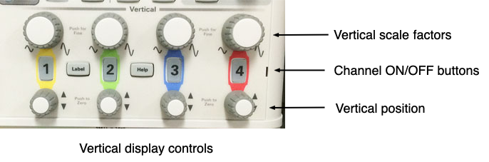
The position of the trace can be adjusted with the small knob just below the illuminated “1” in the Vertical section of the front panel. Try rotating that knob back and forth and observe how the trace, and the ground indicator, move up and down on the screen. The position knobs for the four channels are used to spread the four traces out on the screen so you can see them.
Now let’s look at some signals.
-
Open up the storage compartment on the top of the scope and remove the scope probe that has the yellow markers on the cable. The probes should have colored bands on them, either yellow or green. These are there so when you are using multiple probes you can easily see which probe is associated with each signal trace on the screen.
-
Insert the probe’s connector onto the metal BNC connector for channel one. To make proper contact, the connector needs to be pushed onto the scope’s connector fully and then rotated clockwise to lock it in place. You’ll know it’s locked in place if you can’t pull it off (with a gentle pull) without first rotating it counter-clockwise.
-
At the other end of the cable, the probe has a metal hook at the tip that is exposed by pulling back on the plastic body of the probe. At the lower edge of the scope, hook the probe tip onto the metal tab that says “Probe Comp” just right of the USB port.
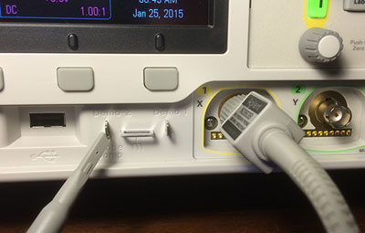
Note 1: The “Probe Comp” metal tab is only used for testing and calibrating the scope. We don’t use it for any of our normal measurements. This is probably the only time this semester that you will be attaching the probe to it.
Note 2: The black ground clip on the probe does not have to be connected to a ground point when the probe is attached to the Probe Comp test point. In all other situations the ground lead must be connected to the circuit ground in order to make measurements.
You should now see two yellow lines going across the screen about a half a grid spacing apart. To get a better view of the signal we need to change the vertical scale factor to make the signal bigger on the screen.
-
In the Vertical section of the front panel, just above the illuminated “1”, the large knob is the vertical scale adjustment. There is one for each channel. Rotate the one for channel 1 a couple of clicks to change the vertical scale factor to 1.0 volts/division (shown at the top left of the display) and this will move the two yellow lines further apart.
You should be able to see a lot of vertical lines running around on the screen between the two horizontal lines. The display should look something like this.
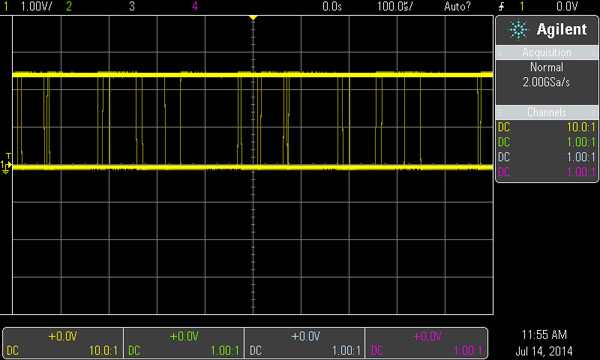
The next step is to get the display to sit still so we can see what it looks like. To do this we need to set up the triggering on the scope. On an oscilloscope, “triggering” means the set of conditions that cause the scope to start drawing a picture of the signals present on its input channels.
Understanding how triggering works and setting up the triggering conditions is probably the most important aspect of making a scope into a useful diagnostic tool.
The scope can be set to trigger when the input signal meets a set of conditions and it will then display the signals on all the channels that occurred before and after that time. It will then wait until the conditions are met again, and then display the signal again. With periodic signals this gives you stable display of the signals since each time they are drawn on the screen they are in the same position. When the scope doesn’t know what to trigger on (like now), it just shows a running (live-stream) display of the incoming signal which usually results in the plot of the signal dancing around on the screen. While you are seeing the signal, it probably won’t be stable on the screen and it will be difficult to analyze. When the triggering has been adjusted properly a stable display will be shown and you can get a clear look at the shape of the signal.
-
In the Trigger portion of the front panel, press the “Trigger” button to bring up the Trigger Menu. The lower edge of the screen now shows labels for the buttons below the screen. Pressing the button below one of the labels will bring up a list of all the possible settings for that option. Note that the one pressed will also have a green circle with an arrow on it. This indicates that the setting can be adjusted using the knob just below the “Trigger” button.
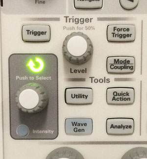
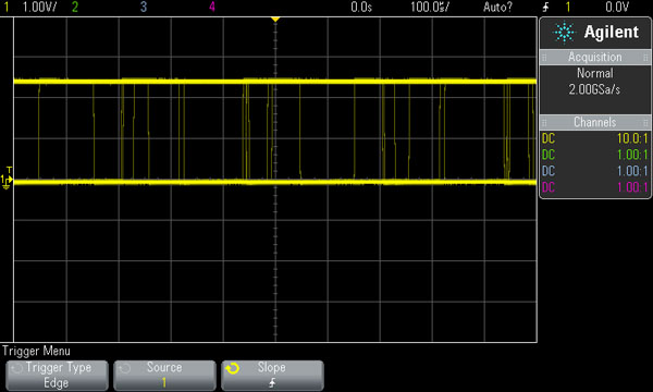
The Trigger Menu consists of the following items.
-
Trigger Type - Determines what type of signal to trigger on. Pressing the button will show all the different triggering types the scope supports. “Edge” triggering is the most common and that’s what we will use today. If it doesn’t say “Edge”’, use the knob to select it.
-
Source - Tells which input channel to use for triggering. Set it to channel 1.
-
Slope - For edge triggering, determines whether to trigger on a signal edge when the signal is going from a low voltage to a high voltage, high to low, either, etc. Set it for a rising edge (little arrow pointing up).
Now that the scope knows to trigger on a rising signal edge on channel 1, we need to tell the scope exactly what voltage level to trigger on. The trigger level is adjusted with “Level” knob in the Trigger section and the value is shown at the top right of the display. Right now it probably says “0.0V” and this is the problem. Since the signal goes from 0 volts to about 2.5 volts, there is no rising edge where it is zero volts so the scope is not triggering. The scope actually tells us that it’s not triggering by putting “Auto?” in the top right of the screen. The question mark is the scope’s way of saying that it’s not triggering.
-
-
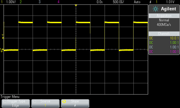
Rotate the Level knob until the value in the upper right says 1.0V and the display should freeze and show something like this. Note that the “Auto?” has changed to “Auto”.
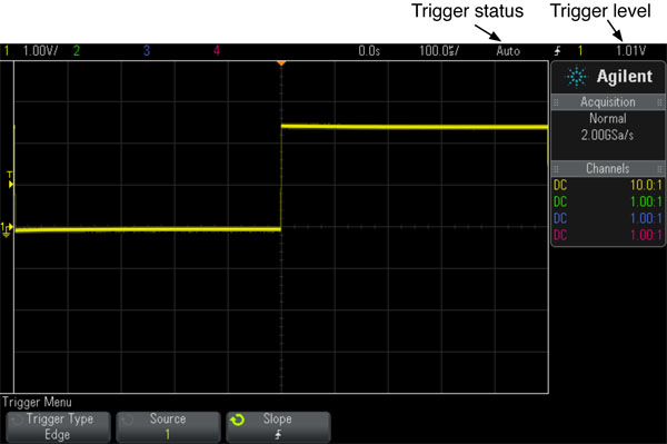
The trigger level is always indicated on the display with the small “T” and triangle along the left side of the display. When the level is being adjusted it also shows it as a horizontal line through the display. Look at the top center part of the display and there should be small solid triangle pointing down. This indicator shows the point along the horizontal (time) axis where the trigger condition was met. The default position is in the middle of the screen so you can see what the signal looked like before and after the triggering occurred.
-
We can change the horizontal position on the screen of the triggering point. In the Horizontal section of the front panel (see below), try rotating the small knob on the right. This is the Horizontal Postion control and the little solid triangle (and the displayed signal) will move right or left on the screen showing more of the signal before or after the trigger point. This can be very useful if you want to see what happened with a signal some time before or after the point where the scope was triggered.
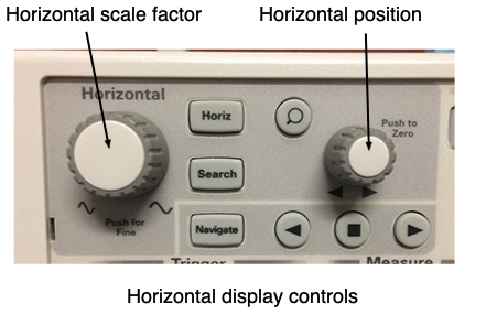
Useful Tip: If the trigger point has been moved left or right so much that it’s not visible on the screen, this is indicated with an empty triangle at the top of the display. You can always return the trigger point to the center of the screen by pressing the horizontal position knob.
-
The last step is to change the horizontal scale factor, also known as the “time base” so we can see more of what the signal looks like. Rotate the large knob in the Horizontal section of the front panel to change the time per division (shown at the top of the display) until it says 500μs. We can now see that the signal is a square wave that repeats every 1000 microseconds, or 1msec. From the vertical scale we can see that the signal goes between zero volts and +2.5 volts.
-
Try playing with the controls (horizontal scale, vertical scale, horizontal position, vertical position, trigger level) to get a feel for how they affect what you see on the screen. Note that using the vertical position control to move the trace up and down on the screen does not affect the triggering level, it moves with the trace.
Generating Signals from the Arduino
In following lab tasks you will use your Arduino to generate a number of signals, and make measurements of these signals using the oscilloscope.
The Arduino Uno is a microcomputer development board based on an Atmel ATmega328P eight-bit microcontroller. Along with the microcontroller the board has connectors to allow solderless connection to the ATmega328P input and output pins, a clock oscillator, a second microcontroller for implementing a USB interface, and other related components. As can be seen below, the Uno has 13 I/O ports along the top that are labeled “Digital (PWM-)”. These are referred to as ports D0 through D13 in the notes below. The six I/O ports at the lower right are labeled “Analog In” on the board and these are referred to as ports A0 through A5 below.
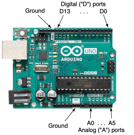
There are also a few places on these connectors where you can make connections to the ground on the Arduino. In all our Arduino lab exercises we will need to use one of these to make sure the Arduino’s ground is connected to the ground on our breadboard or other devices.
In this part of the lab exercise you will be downloading to the Arduino a test program that generates various signals on the Arduino’s output pins. The oscilloscope will then be used to observe these signals and make measurements of them.
In your ee109 folder, create a lab2 folder.
cd Desktop
cd ee109
mkdir lab2
From the class web site download into the lab2 folder the file “lab2.zip” and
extract the contents. You should end up with four files:
-
lab2.o- A binary file containing the program you will download to your Arduino. -
uscid.c- A C file you will use to customize the program in the Arduino. -
Makefile- A Makefile for use with the lab2.o and uscid.c files. -
morse.c- A template file for the Morse code portion of Lab 2. -
Lab2_Answers.txt- A text file that you can edit with your text editor to record your answers to the questions below. This file must be uploaded to Gradescope by the lab due date.
Now that we have the necessary Arduino files in the lab2 folder, we need to build the Arduino program that will generate the signals.
-
Open the
uscid.cfile with your text editor. It only has a couple of lines and should look like this.#define USCID 1234567890 unsigned long long hash = USCID;
-
Use your text editor to change the 10 digit number on the first line to be your USCid number (without any dashes), and then save and close the file. Note: If you are working with partner for this lab, just pick one of the partners USCid number and use that one. You don’t have to repeat the following measurements for each person in the group.
-
Plug one end of the USB cable from your lab kit into the USB connector on the Arduino board, and plug the other end of the cable into a port on your computer. If your computer only has USB-C ports, you will need to buy a USB-A to USB-C adapter.
-
Use your text editor to open the Makefile and check that the OBJECTS line includes both
lab2.oanduscid.oso both files will be used to create the program that will be downloaded to the Arduino. -
As was done in Lab 0 a couple weeks ago, you may have to edit the PROGRAMMER line at the top of the Makefile to make it work on your computer.
Useful tip: In Lab 0 we compiled the program with the command “
make” and then downloaded it with the command “make flash”. If instead you just type “make flash”, the program will check to see if the program needs to be compiled before downloading it. If so, it will do the compile steps as if you had typed “make”, and then it will do the downloading. Only having to type “make flash” each time you want to reprogram the Arduino can speed things up, but also makes it difficult to see if the compiling generated any warnings. -
Type the command “
make flash”. This will build the Lab 2 test program and download the program data to the Uno.
If you previously programmed your Arduino in Lab 0 to make the LED near the D13 I/O pin blink, it was blinking on half the time and off half the time. The “make flash” command you just did to downloaded the Lab 2 program to the Arduino should make the LED now blink a heartbeat pattern about once each second (“blink blink ……. blink blink ……. blink blink …..”). If it’s still blinking the Lab 0 pattern then something has gone wrong and needs to be fixed before proceeding to measure any signals.
Task 2: Measuring Periodic Signals
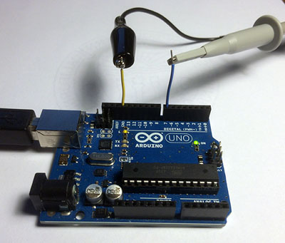
The program in the Arduino is now generating a periodic signal on one of the output pins and we want to observe this signal with the oscilloscope. The microcontroller input and outputs pins are all connected to one of the four black connectors along the edges of the boards. To connect the scope probes to one of these signals,
- Take a short (1-2 inch) piece of wire and strip about 1/4” off each end.
- Insert one end down into the hole in the black connector for the signal you wish to measure.
- Hook the probe clip to the other end of the wire.
- Do the same for the scope probe’s black ground connector so the Arduino’s ground and the scope’s ground are connected together. The wire from the probe’s ground clip should be inserted into one of the ground connections on the board (labeled “GND”).
An example of this is shown in below, however you will be plugging wires into different holes on the connectors than is shown below. The picture below is just an example of how the conenctions can be made.
The Arduino is now generating a period signal that is appearing on port A0. This is a digital signals that transition very rapidly between the two logic states: 0 and 1. When the signal is low (very close to the “Ground” level) it is in the 0 state. When the signal is high, probably about +5V in this case, it is in the 1 state.
Connect the oscilloscope probe to port A0 and adjust the display and trigger settings to get a stable display on the screen. The trigger setting should be same as you used in Part 1 above (Type=Edge, Source=1, Slope=rising). Once the display is stable, you can analyze the timing of the periodic signal. The following measurements need to be made:
-
Time in the 1 state - Use the horizontal scale factor and the grid lines on the screen to determine this. For example if a signal is high for 2.6 divisions and the horizontal scale is set to 200μs per division, then the signal is high for 2.6 × 200μs = 520 μs. Remember to specify the units of time: ms, μs or ns.
-
Time in the 0 state - Same as above but measure when the signal is low.
-
Period - This is the time it take for a periodic signal to repeat. It should be the sum of the time in the 1 state plus the time in the 0 state.
-
Frequency - The frequency of he signal is the inverse of the period. For example, if the period is 2ms, then the frequency is given by

-
Duty cycle - The duty cycle of a signal is the ratio (expressed as a percentage) of the time the signal is in the 1 state (high) to the period of the signal.

Question 1: Enter the results of your measurements for the A0 signal on the paper grading sheet and show the results to one of the teaching staff. They will record on the grading sheet that you completed this task.
Generating Non-Periodic Signals
For the next part of this lab exercise you will build a signaling device that makes an LED flash the Morse code signal for a letter of the alphabet. Rather than have 26 input buttons it will only have three, each assigned to one of three letters of the alphabet. When one of the buttons is pressed, an LED will flash the Morse code signal for the corresponding letter.
Morse Code
Morse code is a method of signaling letters and numbers by sending on and off patterns of light or audible tones. It was first developed in the 1830’s and for many years was the standard way of communicating via telegraph and radio. It is still used today by amateur radio operators, the military, and sometimes for emergency communication.
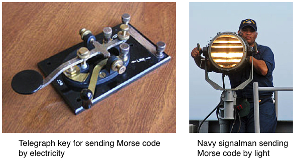
Characters in Morse code consist of a unique set of short or long signals, known as “dots” and “dashes”. The codes for letters A through Z and 0 through 9 are shown below. The dots and dashes of a character are separated by a short gap, and a longer gap separates characters. The most widely known Morse code sequence is the distress call “SOS” of three dots, three dashes, three dots.
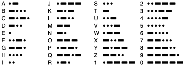
The length in time of a dot or dash in Morse code is not specified directly, only the relationship between the dot and dash length:
- Dashes are three times longer than a dot.
- Gaps between the dots and dashes of a single character are the same length as the dot.
- The gap between characters is the length of the dash.
The speed of the transmission of the characters can cover a wide range, but the above ratios must be adhered to in order to make the transmission understandable by the receiving party.
To see a short video demonstrating the operation of this lab, click here.
Inputs and Outputs
Three buttons will be used as the inputs to the Arduino. These are the same buttons you used in Lab 1. Please refer to the Lab 1 web page for information on how to wire them. The output from the Arduino is using an LED in the same manner as was done in Lab 1.
The three buttons will be used to send the Morse code for the letters ‘U’ (dot-dot-dash), ‘S’ (dot-dot-dot) and ‘C’ (dash-dot-dash-dot).
The Circuit
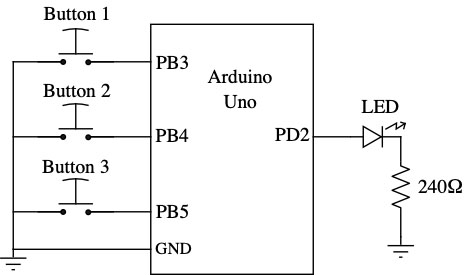
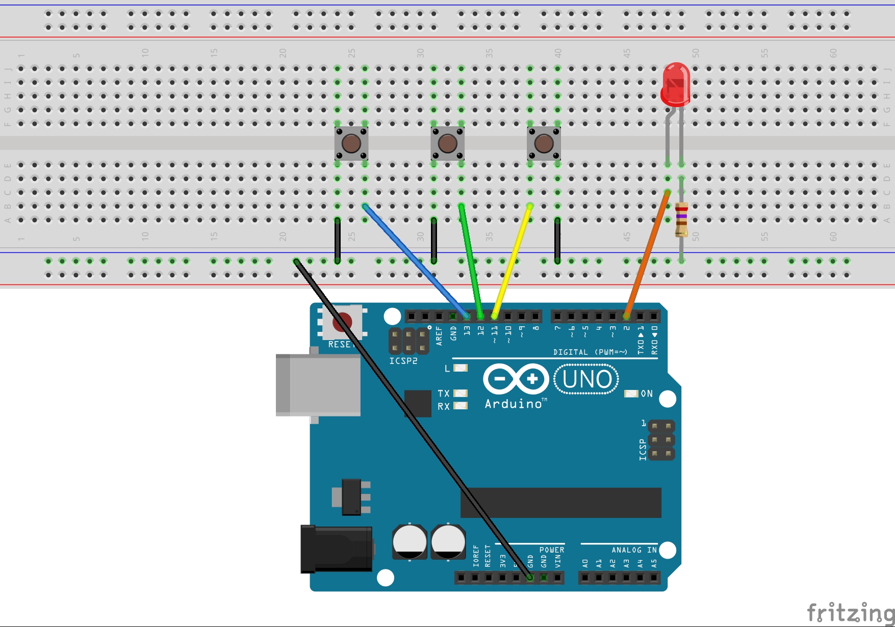
The figures below show a circuit similar to the one you will be building with three buttons for input and an LED for output.
-
The three button inputs are wired to three of the Arduino inputs. The figure below shows them going to D11, D12 and D13, which are connected to Port B, bits 3, 4 and 5 of the microcontroller.
-
The LED and current limiting resistor are connected to one of Arduino outputs. The figure below shows a connection to D2 of the Arduino, which is Port D, bit 2 of the microcontroller.
-
The ground wire from the Arduino to the breadboard goes to one of the rows of holes that forms the buses that runs the length of the breadboard. Use one of the buses by the blue line for ground. The ground connections to the switch and the resistor can all be made to the holes in that bus row.
The Program
For this part of Lab 2, you will need to finish the code for the morse.c file.
This file is provide for you in two forms.
-
The
morse.cfile that is in thelab2.zipfile that you downloaded previously -
A paper copy of the file available from the table in front of the VHE 205 podium. This is the copy you must work with first.
If you examine the program you will note several places where code has been removed and replaced with underlines. Your task is to determine what code should be in all the missing places and complete the program on the paper copy. The basic structure of the program is as follows:
-
Initialization: Lines at the top are used to initialize the registers that control the Port bits for input and output.
-
Main Loop: Each time around the
whileloop, the program checks each input bit connected to a button to see if the button has been pressed. If so, the program generates the correct pattern of flashes to send that Morse code letter. -
flash_led: This routine is called to make the LED light up for a specified length of time and then turn off. -
checkInput: This routine is called to check the state of one of the input bits that the buttons are connected to.
Once you have finished filling in the blank areas of the program, show it to one of the teaching staff so they can review it. If the staff approve of your code, proceed with the following steps.
-
Using your text editor, edit the
morse.cfile to replace all the underlines with the code you developed on paper in the step above. - Edit the
Makefileto change the OBJECTS line so themorse.cfile will be compiled when building the program.OBJECTS = morse.o
-
If the program compiles with no errors, connect your Arduino to your computer and download the program with the
make flashcommand. -
Try pressing each of the buttons and confirm that the LED flashes the correct Morse code pattern for the ‘U’, ‘S’ and ‘C’ letters.
- You also need to check that there is a gap between consectutive letters. Try pressing the ‘S’ button and holding it down to send multiple ‘S’ signals. The LED should flash a distinct pattern for each: “dot-dot-dot”, a gap, “dot-dot-dot”, a gap, etc. The LED should not flash “dot-dot-dot-dot-dot-dot…” with no gap between the letters.
Show the operation of your Morse code sending device to one of the teach staff and they will record on the grading sheet that you completed this task.
Task 3: Observing Non-Periodic Signals
In the task above you programmed the Arduino to produce the Morse code symbols in response to a button being pressed. Unlike the signal you observed earlier in the lab exercise this output signal was “non-periodic” meaning that it doesn’t repeat over and over. The techniques used earlier to observe a periodic signal on the oscilloscope won’t work for looking at non-periodic signals
For this task you will configure the scope to watch for a non-periodic event, one that only happens occasionally, as opposed to the repetitive periodic signals we have observed earlier in this lab. Being able to look at signals that only change occasionally can be very useful when debugging a digital system. To see signals like these the scope has to take a single acquisition of the signal and then hold it so it can be viewed.
For this lab exercise we want to look a the output signal for ‘C’ character “dash-dot-dash-dot” to confirm that is generated correctly. At the start of this lab we specified the timing requirement for correctly sending the dots and dashes of Morse code characters.
- Dashes are three times longer than a dot.
- Gaps between the dots and dashes of a single character are the same length as the dot.
Follow the steps below to configure the scope to capture a non-periodic signal.
-
Turn on the scope and connect the two probes to channels 1 and 2.
-
Turn on both channels by pressing the ‘1’ and ‘2’ buttons until they are lit.
-
Set the vertical controls for both channels for 2 volts/division.
-
Use the vertical position controls to put the yellow channel 1 line in the upper part of the display just above the center of the screen, and the green channel 2 line in the bottom part.
-
Set the horizontal control to 500ms per division. This can be changed later to get a good view of signals.
-
Hook the oscilloscope ground connection to the ground on your breadboard.
-
Channel 1 will be used to view the button press signal. Connect probe 1 to the ‘C’ button output where the wire is going to the input bit for the ‘C’ character.
-
Channel 2 will show the output signal going to the LED. Connect probe 2 to the anode of the LED where the wire from the output bit is connected to the LED. Make sure you have the scope probe connected directly to the output port and not after the LED or the resistor.
-
You need the scope to trigger when the button is pressed so adjust the trigger settings so the scope triggers on a falling edge on channel 1. Press the “Trigger” button in the Trigger section of controls and use the buttons below the screen and the Trigger Level knob to make these settings:
- Set “Trigger Type” to “Edge”.
- Set “Source” to “1”.
- Set “Slope” to a falling edge.
- Adjust the trigger level to about 2 volts.
-
The scope is now be ready to trigger when the ‘C’ button is pressed. Press the “Single” button in the upper right to make it wait for the next trigger signal, and then press the ‘C’ button on your breadboard.
-
If everything is working, you will get a display like that below. The yellow trace is showing the signal from the button you pressed. The green trace is showing the Arduino outputting the Morse code for the ‘C’. Use the horizontal controls to adjust the scope timing and position to get a good view of the signal. Check that the timing is correct for the dots, dashes and the gaps between them.
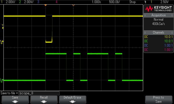
Show the scope display of the ‘C’ character to one of the teaching staff and they will record on the grading sheet that it is being generated correctly.
Task 4: Measuring the Propagation Delay
In Lab 1 we built a simple combinational circuit with a button, NOT gate and LED output. When the input to the NOT gate changes due to the button being pressed, the output changes in response. The time it takes for an output to change in response to an input changing is called the “propagation delay. The length of the propagation delay is specified in the data provided by the manufacturer of the gate, or it can be measured using an oscilloscope. If we had measured the NOT gate’s delay it is around 5ns and is fairly consistant each time the NOT gate input change.
In our circuit this week using software to turn the LED on the there is also a delay from when the button is pressed and the LED first lights up. We now want to measure this delay time to see how it compares to the NOT gate’s delay time.
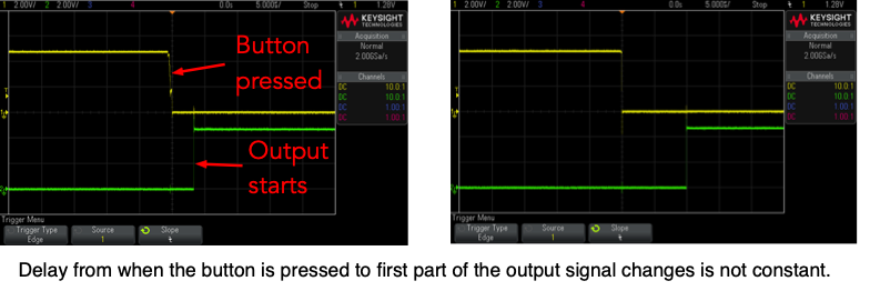
Repeat the experiment done above to show the ‘C’ output, but increase speed of the horizonal timing so any delay between the button on channel 1 and the output on channel 2 can be observed. You probably need to adjust the horizonal speed to around 5μs in order to see the delay as shown below.

Once you have the scope set to where you can see the delay, repeat the action of pressing the button and acquiring the ‘C’ signal 10 times and record the amount of delay for each trial. These delays will likely be much longer, on the order of 1-10 microseconds. That is about two orders of magnitude difference. Software takes much longer because our loop is composed of many software instructions that the processor must fetch from memory, decode and then execute. You can see that if computation needs to be done quickly, hardware has advantages!
Unlike the delay through the NOT gate, these delays also may not be consistant and will vary every time the button is pressed as shown in the two pictures below where the image on the left shows a delay of about 3μs while the one on the right shows a delay around 10μs.
Question 2: Show the results of capturing 10 samples of the propagation delay to one of the teaching staff. and they will record on the grading sheet that you completed this task.
In a review problem below you are asked to explain why the propagation delays vary from one test to another. Think about the process the program goes through to monitor the state of the button and decide whether or not to send the signal to the LED. Hint: ignore the hardware propagation delays which are very small (tens of ns), and think about how your program executes.
Results
The Makefile, morse.c file and the “Lab2_Answers.txt” file with the answers to the review questions edited into it should be uploaded to the Gradescope web site
by the due date. Use the link on Brightspace for Lab 2 to submit your results.
Review Questions
Answer the following questions in your “Lab2_Answers.txt”.
-
Suppose you wanted to measure the frequency of a note played by a piano and sensed from a microphone connected/viewed on an oscilloscope. Answer the following True/False questions with a brief explanation.
- T/F: To measure the frequency, the vertical scale of the oscilloscope would be of more use than the horizontal scale.
- T/F: Since the note is played for a short time period, we should set the triggering to "Single" rather than "Run".
- T/F: If the signal ranges between 0V and 2.5V, the trigger level should ideally be set around 1.25V.
-
If you have used the Horizontal Position control to move the trigger point horizontally so much that you can no longer see the trigger point on the screen, what is the quick way to restore the trigger point back to the middle of the screen?
-
Suppose our design for the Morse code generator had the three buttons on group D, bits 5-3, with the LED attached to group D, bit 2. Assuming appropriate
DDRDvalues, consider the following method of turning on the LED.PORTD = 0x04; // turn on the LEDExplain the problem with this approach and, in particular, what would stop working after the execution of that line of code.
-
In Task 4 above you measured the propagation delay from the button press to the output starting. Can you explain why the propagation delays vary from one test to another? Hint: ignore the hardware propagation delays which are very small (tens of ns), and think about how your program executes.