Due by Friday, November 22nd. Please note that there is NO lab instruction/lecture this week, just the asynchronous assignment. You are welcome to attend your regular lab section to get checked off next week (11/18-11/22), however!

Amortized Analysis

1 - What is amortized runtime?

So, we’ve learned about runtime notations like Big-O, Theta, and Big Omega. But how did we calculates these running time bounds? That lies in the runtime analysis. The majority of the analysis we have done thus far has been about the worst case. However, as we have learned, the worst-case doesn’t always give us an accurate picture of the runtime associated with a data structure or algorithm (ex. hash tables, quicksort).

This is where amortized runtime comes in! Amortized runtime isn’t about the singularly worst time a thing will perform; rather, it’s about how the thing performs averagely on the whole, i.e. “worst-case average-case”. Amortized analysis is specifically used to judge data structures/algorithms that may occasionally have a slow operation, but are on the whole pretty fast.

2 - Amortized Analysis Methods

So we now know the benefits of amortized analysis. Yay! …But how do we do it? How do we take the good (and the bad) times into account accurately?

There are 3 main methods for calculating the amortized analysis of a function. To illustrate the 3, we will consider incrementing a binary counter.

For example, our counter may start with the value: 00000. How expensive is it to increment the counter, i.e. how many operations are necessary? Well, for our first increment, we only need to flip one bit: 00000 –> 00001. But for the next operation, we need to flip two bits: 00001 –> 00010. Say we want to increment the counter again. This time the operation only requires flipping one bit: 00010 –> 00011.

What would we say the runtime of this binary counter increment function is??? As we can see, not every increment operation is the same cost.

2.1 - The Aggregate Method

Using the aggregate method, we will determine the upper bound T(n) on the total cost of a sequence of n operations, then divide it by n to find the average runtime per operation.

For our binary counter, let’s consider incrementing it n times. How many bit flips will be required overall?

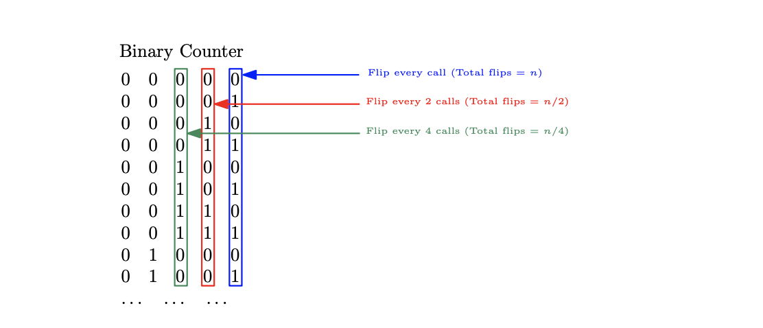
Well, writing out a couple of the increments, we can notice a pattern. The least significant bit will be flipped every single time we increment the counter; so, if we have n increments, then we will flip this bit n times.

The second least signficant bit will be flipped every other increment, so that will be a total of n/2 times.

The thirs bit will be flipped every fourth increment, so that will be a total of n/4 times. Notice a pattern?

The upper bound T(n) then will be the summation of all of these flips, since we want the total cost of our n operations.

This summation will be:

Thus, T(n) is equal to 2n. Now, to find the average runtime per operation, we must divide it by n. So our final amortized cost is 2n / n = 2.

Thus, the increment function for our binary counter has a constant-time amortized cost!

2.2 - The Accounting (Piggy Bank) Method

Could we find this amortized cost another way? The idea behind the accounting (piggy bank) method is that we allocate a fixed cost to each call of the function. Cheap calls will then accrue a saved amount, and expensive calls will dip into this saved fund. The expensive calls are payed off by the cheaper ones before it.

Continuing with the binary counter example, let’s use the accounting method to determine the amortized runtime.

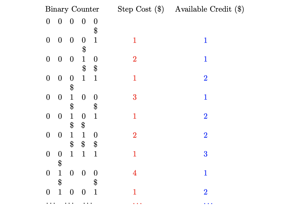
First, we need to set our fixed cost at the beginning that is high enough for low-cost operations to have a little left over. Let’s start with a fixed cost of $2.

Flipping a bit costs $1.

For our first increment from 00000 -> 00001, then we pay $2 to do the operation.

We get to save $1.

For the next increment 00001 -> 00010, we deposit $2 to do the operation.

We end up using both of those dollars to do 2 flips; we still have $1 saved from our first cheap operation.

For the next increment 00010 -> 00011, we pay our $2.

We end up only having to use $1 for a flip.

We now have $2 saved.

For the next increment 00011 -> 00100, we pay $2.

For this increment, we end up having to use $3 to execute the number of flips we need.

Luckily, we have $2 saved from cheap operations.

We’re left with $1 in the bank.

Because we never overspend our savings (i.e. our fixed cost of $2 is always enough, no matter what) then we can see that our increment function will have a constant time amortized cost! If instead the amount of money per operation was linear and not a fixed value (ex. the amount we had to pay was dependent on what number of increments we were doing), then we’d be able to determine that the amortized runtime is linear.

Basically, with this method, you want to find the smallest amount of money possible that always keeps your savings >= 0. If that value is constant, then the amortized cost of the function is constant; if that value is a variable like n, then the amortized cost of the function is linear; if that value is a variable like n^2, then the amortized cost of the function is quadratic, etc.

2.3 - The Potential Method

The potential method is good for tracking more complex problems, that may not have as definitive start and end points.

WIth this method, we define a function Φ that maps the state of our data structure (ex. the state 01011 for our binary counter) to a non-negative number. Say “S” is the state of our data structure; Φ(S) can be thought of as a value that will calculate the amount of “potential” that state has, similar to physics. An operation (ex. an increment) will move us from one state to another state, which will change the potential.

If the operation costs c, then the amortized cost A will be:

A := c + (Φ(S1) - Φ(S0))

Where Φ(S1) is the value of the potential function for the state we moved to, and Φ(S1) is the value of the potential function we were originally in.

How do we define Φ(S) in this problem? Φ(S) will be equal to the number of ones present in the state of the counter.

Great! We have our potential function- now what? We calculate the amortized cost. If changing from from S0 to S1 requires us to flip f bits, then f-1 of these flips will be from 1 –> 0, and the last one will be 0 –> 1. (Try it out with some examples!). This means the number of ones present in the new state will be f-2.

The amortized cost will then be:

A = f - (f-2) = 2

Which is a constant, so the amortized runtime is constant! The potential method is one of the trickiest methods to understand because of how abstract it is. For more help on this topic, I have personally found these notes to be very helpful (it is where I pulled this explanation from!).

3 - Stack/Queue Assignment

For this week’s lab, you will be implementing a queue with two stacks, just like problem 3 of written homework 5 describes. There are two functions you need to implement: front() and dequeue(). Front returns the value at the front of the queue. Dequeue removes the item at the front of the queue.

For a starting point on how to do this, refer to the note in homework 4:

”””

It is possible to implement a queue using two stacks stack1 and stack2, by implementing the functions in the following manner:

enqueue(x): push x on stack1.

dequeue(): if stack2 is not empty, then pop from it. Otherwise, pop the entire contents of stack1, pushing each one onto stack2. Now pop from stack2.

”””

Once you have implemented both functions, all tests should pass when running “make” in Docker. Optionally, there is a commented-out stress test, that you can see if you also pass. Note that this test takes usually a minute or two to complete, and it is not necessary for check off!

Image credits go to University of Hawaii Analysis of Algorithms Fall 2019 Lecture 1 Notes.