***
←
→
Machine Learning
[ALSO, search(ing) for PATTERNS]
|
Types of AI
Here is a good way [after Arend Hintze] to classify AI types (not just techniques!)..
Type I: Reactive machines - make optimal moves - no memory, no past 'experience'.
Type II: Limited memory - human-compiled , one-shot 'past' 'experiences' are stored for lookup.
Type III: Theory of Mind - "the understanding that people, creatures and objects in the world can have thoughts and emotions that affect the AI programs' own behavior".
Type IV: Self-awareness - machines that have consciousness, that can form representations about themselves (and others).
Type I AI is simply, application of rules/logic (eg. chess-playing machines).
Type II AI is where we are, today - specifically, this is what we call 'machine learning' - it is "data-driven AI"! Within the last decade or so, spectacular progress has been made in this area, ending what was called the 'AI Winter'.
As of now, types III and IV are in the realm of speculation and science-fiction, but in the general public's mind, they appear to be certainty in the near term :)
What is ML?
Machine learning focuses on the construction and study of systems that can learn from data to optimize a performance function, such as optimizing the expected reward or minimizing loss functions. The goal is to develop deep insights from data assets faster, extract knowledge from data with greater precision, improve the bottom line and reduce risk.
- Wayne Thompson, SAS
Types of ML
The following notes are from various sources..
There are broadly, three 'flavors' of AI:
- Symbolic reasoning (RULES-driven)
- Reinforcement learning (REWARDS-driven)
- Machine learning (DATA-driven) ['ML']
The key types of ML include:
- Supervised learning - using all labeled data
- Semisupervised learning - using partially labeled data
- Unsupervised learning - using unlabeled data
Supervised learning algorithms are "trained" using examples where in addition to features [inputs], the desired output [label, aka target] is known.
Unsupervised learning is a type of machine learning where the system operates on unlabeled examples. In this case, the system is not told the "right answer." The algorithm tries to find a hidden structure or manifold in unlabeled data. The goal of unsupervised learning is to explore the data to find intrinsic structures within it using methods like clustering or dimension reduction.
For Euclidian space data: k-means clustering, Gaussian mixtures and principal component analysis (PCA)
For non-Euclidian space data: ISOMAP, local linear embedding (LLE), Laplacian eigenmaps, kernel PCA.
Use matrix factorization, topic models/graphs for social media data.
Here is a WIRED mag writeup on unsupervised learning:
Let's say, for example, that you're a researcher who wants to learn more about human personality types. You're awarded an extremely generous grant that allows you to give 200,000 people a 500-question personality test, with answers that vary on a scale from one to 10. Eventually you find yourself with 200,000 data points in 500 virtual "dimensions" - one dimension for each of the original questions on the personality quiz. These points, taken together, form a lower-dimensional "surface" in the 500-dimensional space in the same way that a simple plot of elevation across a mountain range creates a two-dimensional surface in three-dimensional space.
What you would like to do, as a researcher, is identify this lower-dimensional surface, thereby reducing the personality portraits of the 200,000 subjects to their essential properties - a task that is similar to finding that two variables suffice to identify any point in the mountain-range surface. Perhaps the personality-test surface can also be described with a simple function, a connection between a number of variables that is significantly smaller than 500. This function is likely to reflect a hidden structure in the data.
In the last 15 years or so, researchers have created a number of tools to probe the geometry of these hidden structures. For example, you might build a model of the surface by first zooming in at many different points. At each point, you would place a drop of virtual ink on the surface and watch how it spread out. Depending on how the surface is curved at each point, the ink would diffuse in some directions but not in others. If you were to connect all the drops of ink, you would get a pretty good picture of what the surface looks like as a whole. And with this information in hand, you would no longer have just a collection of data points. Now you would start to see the connections on the surface, the interesting loops, folds and kinks. This would give you a map.
Semisupervised learning is used for the same applications as supervised learning. But this technique uses both labeled and unlabeled data for training - typically, a small amount of labeled data with a large amount of unlabeled data. The primary goal is unsupervised learning (clustering, for example), and labels are viewed as side information (cluster indicators in the case of clustering) to help the algorithm find the right intrinsic data structure. image analysis - for example, identifying a person's face on a webcam - textual analysis, and disease detection.
With reinforcement learning, the algorithm discovers for itself which actions yield the greatest rewards through trial and error. Reinforcement learning has three primary components:
1. agent - the learner or decision maker
2. environment - everything the agent interacts with
3. actions - what the agent can do
The objective is for the agent to choose actions that maximize the expected reward over a given period of time. The agent will reach the goal much quicker by following a good policy, so the goal in reinforcement learning is to learn the best policy. Reinforcement learning is often used for robotics and navigation.
Markov decision processes (MDPs) are popular models used in reinforcement learning. MDPs assume the state of the environment is perfectly observed by the agent. When this is not the case, we can use a more general model called partially observable MDPs (or POMDPs).
Common ML algorithms
To reiterate, these are the most common ML algorithms:
- Linear Regression
- Logistic Regression
- Decision Trees
- SVM
- Naive Bayes
- KNN
- K-Means Clustering
- Random Forest
- Gradient Boost, Adaboost
- Neural nets ("NN, ANN, DNN, CNN, RNN..")
Since we already looked at Linear Regression through Adaboost in the context of DM, we'll now focus just on neural nets, for machine learning (this is also the industry trend!).
Algorithm: Neural nets! ['NN']
A form of 'AI' - use neuron-like connected units that store learning (training) data that has known outcomes, use it to be able to gracefully respond to new situations (non-training, 'live' data) - like how humans/animals learn!
Neural networks (NNs) can be used to:
- recognize/classify features - traffic, terrorists, expressions, plants, words..
- detect anomalies - unusual CC activity, unusual machine states, gene sequences, brain waves..
- predict exchange rates, 'likes'..
As you can imagine, 'Big Data' can help in all of the above! The bigger the training set, the better the learning (more conditions, more features), better the result.
Algorithm: NN [cont'd] [the rundown!]
Below is an overview of how NNs work..
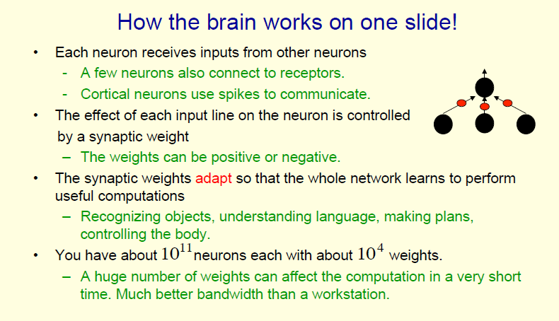
The brain (specifically, learning/training) is modeled after strengthening relevant neuron connections - neurons communicate (through axons and dendrites) dataflow-style (neurons send output signals to other neurons):
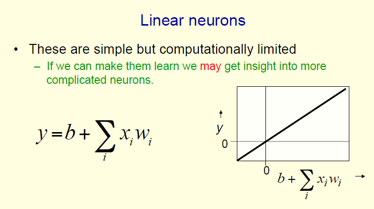
Linear (identity), 'leaky' output: input values get passed through 'verbatim' (not very useful to us, does not happen in real brains!):
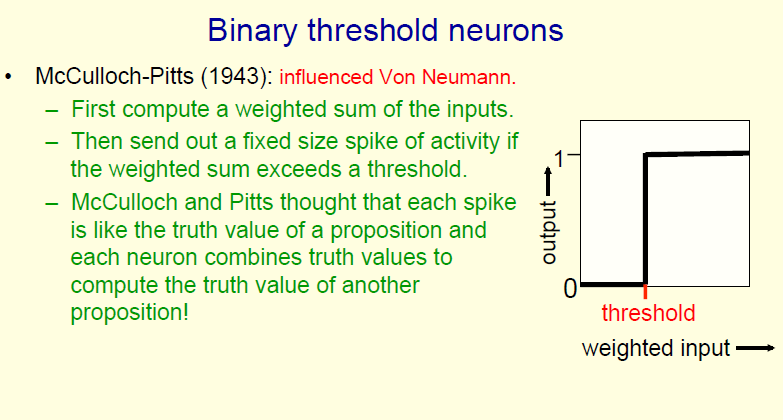
A better model is when a neuron outputs a 1 (stays 0 to start with) ("fires") if and when its combined inputs exceed a threshold value:
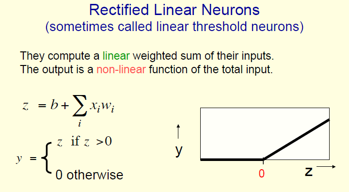
Another option is to convert the 'step' pulse to a ramp:
Even better - use a smoother buildup of output:
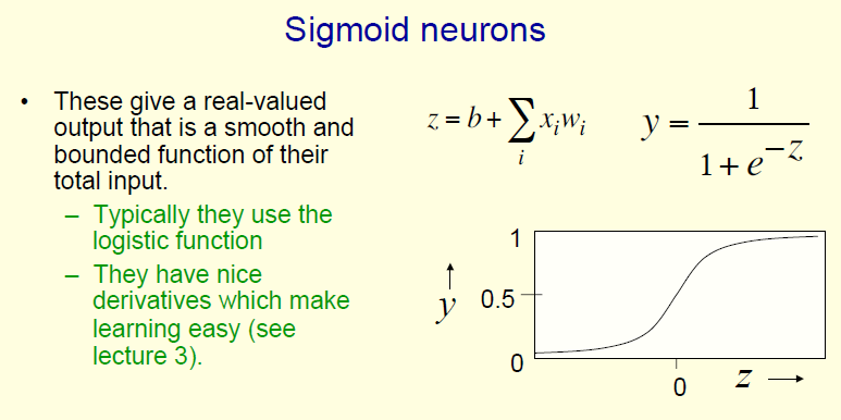
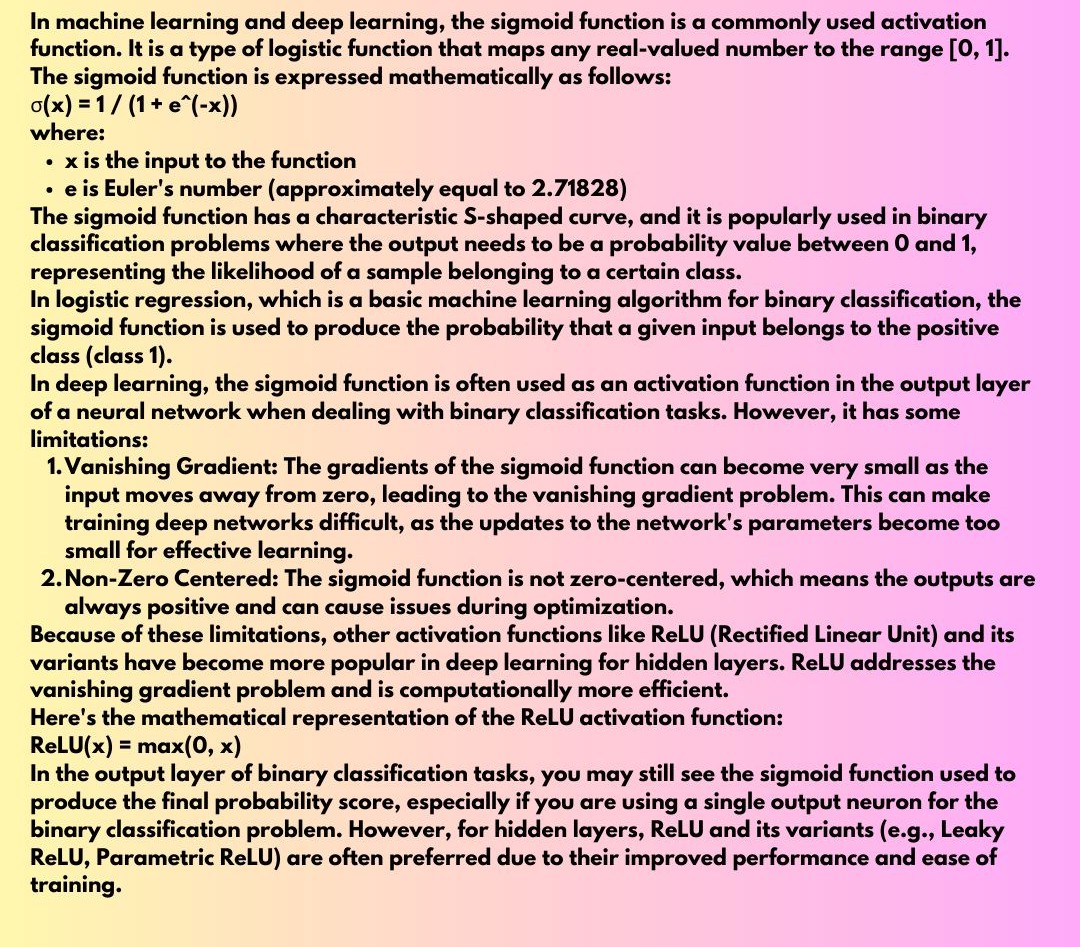
*Even* better - use a sigmoidal probability distribution for the output:
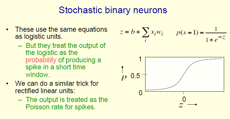
The functions we use to generate the output, are called activation functions - the ones we looked at are identity, binary threshold, rectifier and sigmoid. The gradients of these functions are used during backprop. There are more (look these up later) - symmetrical sigmoid, ie. hyperbolic tangent (tanh), soft rectifier, polynomial kernels...
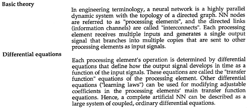
This is from an early ('87) newsletter - today's NNs are not viewed as systems of coupled ODEs - instead we use 'training' to make processing element 'learn' how to respond to its inputs:
With the above info, we can start to build our neural networks!
* we create LAYER upon LAYER of neurons - each layer is a set (eg. column) of neurons, which feed their (stochastic) outputs downstream, to neurons in the next (eg. column to the right) layer, and so on
* each layer is responsible for 'learning' some aspect of our target - usually the layers operate in a hierarchical (eg. raw pixels to curves to regions to shapes to FEATURES) fashion
* a layer 'learns' like so: its input weights are adjusted (modified iteratively) so that the weights make the neurons fire when they are given only 'good' inputs.
Here is how to visualize the layers.
The above steps can be summarized this way:
Learning (ie. iterative weights modification/adjustment) works via 'backpropagation', with iterative weight adjustments starting from the last hidden layer (closest to the output layer) to the first hidden layer (closest to the input layer). Backpropagation aims to reduce the ERROR between the expected and the actual output [by finding the minimum of the [quadratic] loss function], for a given training input. Two hyper/meta parameters guide convergence: learning rate [scale factor for the error], momentum [scale factor for error from the previous step]. To know more (mathematical details), look at this, and this.
To quote MIT's Alex "Sandy" Pentland: "The good magic is that it has something called the credit assignment function. What that lets you do is take stupid neurons, these little linear functions, and figure out, in a big network, which ones are doing the work and encourage them more. It's a way of taking a random bunch of things that are all hooked together in a network and making them smart by giving them feedback about what works and what doesn't. It sounds pretty simple, but it's got some complicated math around it. That's the magic that makes AI work."
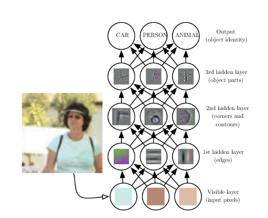
As per the above, here is a schematic showing how we could look for a face:
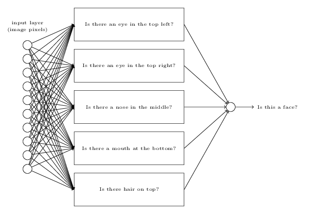
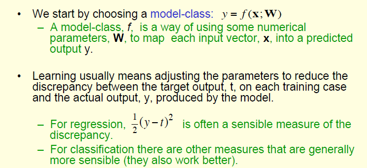
Note that a single neuron's learning/training (backprop-based calculation of weights and bias) can be considered to be equivalent to multi-linear regression - the neuron's inputs are features (x_0, x_1..), the learned weights are corresponding coefficients (w_0,w_1..) and the bias 'b' is the y intercept! We then take this result ('y') and non-linearize it for output, via an activation function. So overall, this is equivalent to applying logistic regression to the inputs. When we have multiple neurons in multiple layers (all hidden, except for inputs and outputs), we are chaining multiple sigmoids, which can approximate ANY continuous function! THIS is the true magic of ANNs. Such 'approximation by summation' occurs elsewhere as well - the Stone-Weierstrass theorem, Fourier/wavelet analysis, power series for trig functions...
A simpler example - a red or blue classifier can trained, by feeding it a large set of (x,y) values and corresponding up or down expectations - the learned weights in this case are the coefficients A and B, and the learned bias is C, in the line equation Ax+By=C [equivalently, m and c, in y=mx+c]:
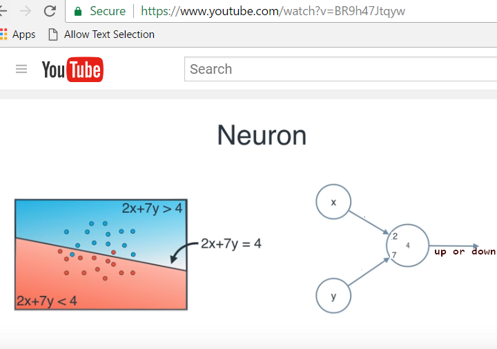
In other words: we feed in a large set of (x,y) values taken from above and below our line, feed it to the neuron and ask, "up, or down"? Depending on its response in relation to the correct one, we nudge the two weights and the bias repeatedly, till the correct ones are learned: 2,7,4.
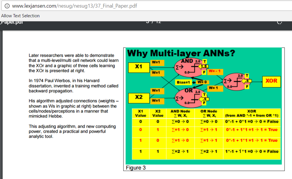
Here is a simple network to learn XOR(A,B) - here all the 6 weights (1,1,1,1,-1,1) are learned:
The following clip shows how a different NN (with one middle ('hidden') layer with 5 neurons) learns XOR - as the 5 neurons' weights (not pictured) are repeatedly modified, the 4 inputs ((0,0), (0,1), (1,0), (1,1)) progressively lead to the corresponding expected XOR values of 0,1,1,0 [in other words, the NN learns to predict XOR-like outputs when given binary inputs, just by being provided the inputs as well as expected outputs]:
Again - how a single neuron works
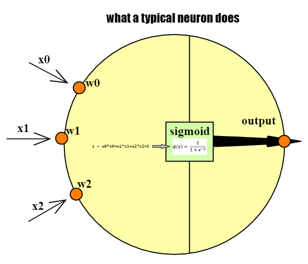
Sigmoid
NN++ : Deep Learning!
Deep Learning is starting to yield spectacular results, to what were once considered intractable problems..
Why now? Massive amounts of learnable data, massive storage, massive computing power, advances in ML.. Here is NVIDIA's response (to 'why now')..
In Deep Learning, we have large numbers (even 1000!) of hidden layers, each of which learns/processes a single feature.
Eg. here is a (non-so-deep) NN:
"Deep learning is currently one of the best providers of solutions regarding problems in image recognition, speech recognition, object recognition, and natural language with its increasing number of libraries that are available in Python. The aim of deep learning is to develop deep neural networks by increasing and improving the number of training layers for each network, so that a machine learns more about the data until it's as accurate as possible. Developers can avail the techniques provided by deep learning to accomplish complex machine learning tasks, and train AI networks to develop deep levels of perceptual recognition."
Q: so what makes it 'deep'? A: the number of intermediate layers of neurons.
Deep learning is a "game changer"..
DNN: on GPUs!
GPUs (multi-core, high-performance graphics chips made by NVIDIA etc.) and DNNs seem to be a match made in heaven!
NVIDIA has made available a LOT of resources related to DNNs using GPUs, including a framework called DIGITS (Deep Learning GPU Training System). NVIDIA's DGX-1 is a deep learning platform built atop their Tesla P100 GPUs. Here is an excellent intro' to deep learning - a series of posts. Here is a GPU-powered self-driving car (with 'only' 37 million neurons) :)
Microsoft has created a GPU-based network for doing face recognition, speech recognition, etc.
IBM has its SyNAPSE chip, and TrueNorth NN chip.
FPGAs also offer a custom path to DNN creation.
Also: TeraDeep, CEVA, Synopsis, Alluviate..
[aside] Convolution: a signal-processing operation
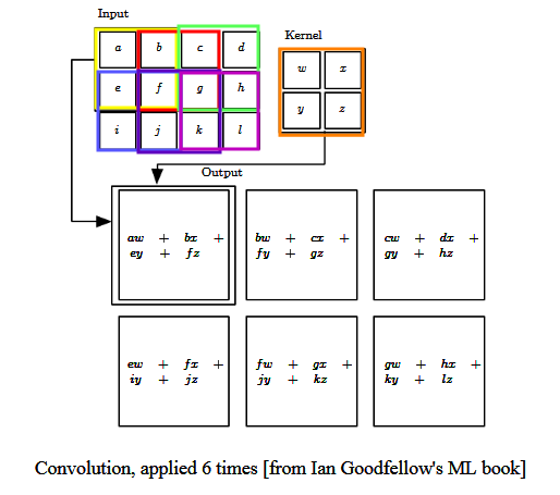
A convolution is a blending (or integrating) operation between two functions (or signals or numerical arrays) - one function is convolved (pointwise-multiplied) with another, and the results summed.
Here is an example of convolution - the 'Input' function [with discrete array-like values] is convolved with a 'Kernel' function [also with a discrete set of values] to produce a result; here this is done six times:
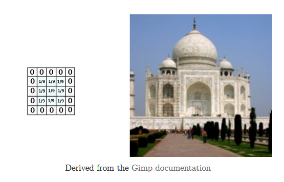
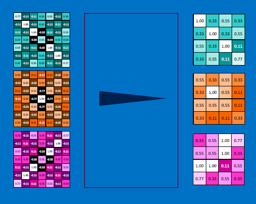
Convolution is used heavily in creating image-processing filters for blurring, sharpening, edge-detection, etc. The to-be-processed image represents the convolved function, and a 'sliding' "mask" (grid of weights), the convolving function (aka convolution kernel):
Here is [the result of] a blurring operation:
Here you can fill in your own weights for a kernel, and examine the resulting convolution.
So - how does this relate to neural nets? In other words, what are CNNs?
CNN (Convolutional Neural Network, aka ConvoNet)
CNNs are biologically inspired - (convo) filters are used across a whole layer, to enable the entire layer as a whole to detect a feature. Detection regions are overlapped, like with cells in the eye.
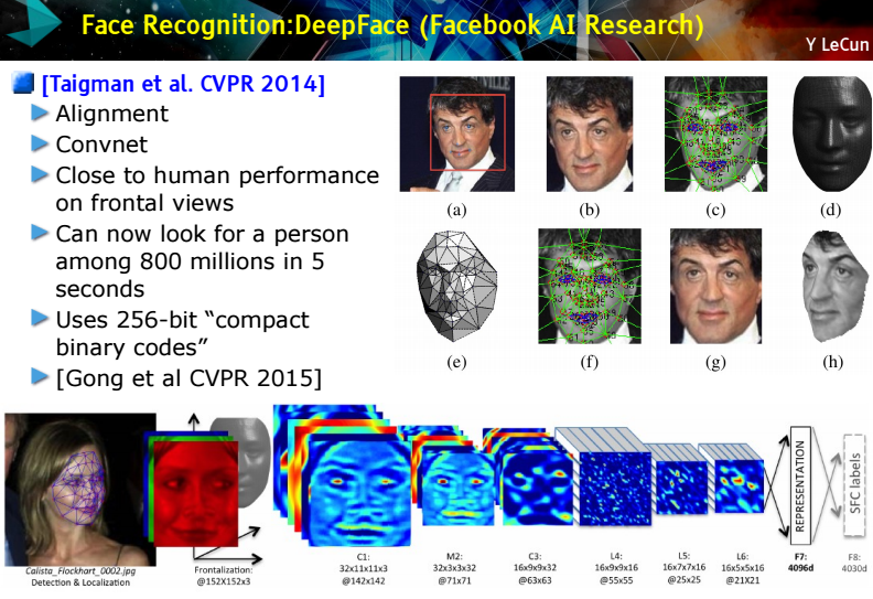
Here is an*excellent* talk on CNNs/DNNs, by Facebook's LeCun.
Here is a *great* page, with plenty of posts on NNs - with lots of explanatory diagrams.
CNN [cont'd]
In essence, a CNN is where we represent a neuron's weights as a matrix (kernel), and slide it (IP-style) over an input (an image, a piece of speech, text, etc.) to produce a convolved output.
In what sense is a neuron's weights, a convolution kernel?
We know that for an individual neuron, its output `y` is expressed by
`y = x_0*w_0 + w_1*x_1 + .... + w_n*x_n + b`, where the `w_i`s represent the neuron's weights, and the `x_i`s, the incoming signals [`b` is the neuron's activation bias]. The multiplications and summations resemble a convolution! The incoming 'function' is `[x_0, x_1, x_2, .... x_n]`, and the neuron's kernel 'function', `[w_0, w_1, w_2, .... w_n]`.
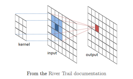
Eg. if the kernel function is `[0,0,0...w_0,w_1,0,0...]` [where we only process our two nearest inputs], the equivalent network would look like so [fig from Chris Olah]:
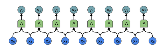
The above could be considered one 'layer' of neurons, in a multi-layered network. The convolution (each neuron's application of `w_0` and `w_1` to its inputs) would produce the following:
`y_0 = x_0*w_0 + x_1*w_1 + b_0`
`y_1 = x_1*w_0 + x_2*w_1 + b_1`
`y_2 = x_2*w_0 + x_3*w_1 + b_2`
....
Pretty cool, right? Treating the neuron as a kernel function provides a convenient way to represent its weights as an array. For 2D inputs such as images, speech and text, the kernels would be 2D arrays that are coded to detect specific features (such as a vertical edge, color..).
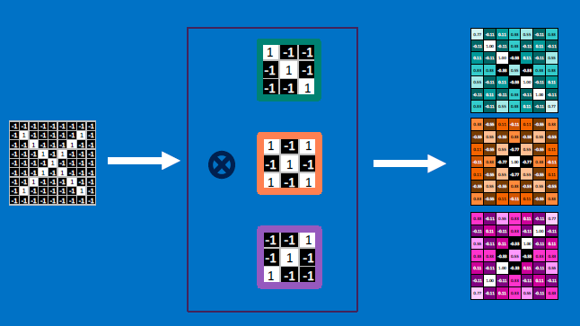
EACH NEURON IS CONVOLVED OVER THE ENTIRE INPUT (again, IP-style), AND AN OUTPUT IS GENERATED FROM ALL THE CONVOLUTIONS. The output gets 'normalized' (eg. clamped), and 'collapsed' (reduced in size, aka 'pooling'), and the process repeats down several layers of neurons: input -> convolve -> normalize -> reduce/pool -> convolve -> normalize -> reduce/pool -> ... -> output.
The following pics are from a talk by Brandon Rohrer (Microsoft).
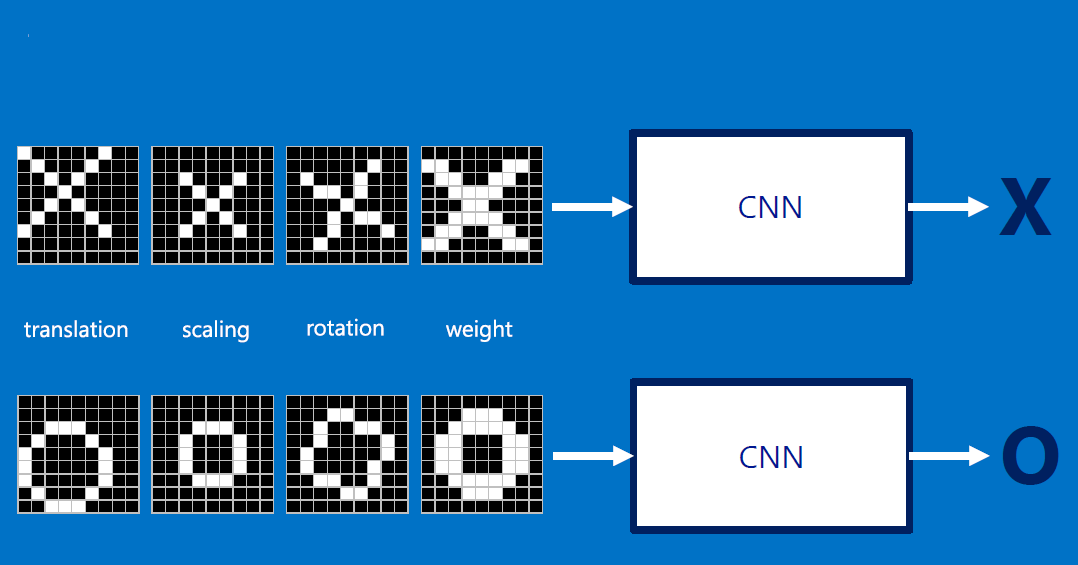
What we want:
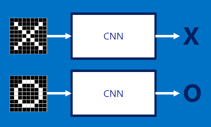
The input can be RST (rotation, scale, translation) of the original:
How can we compute similarity, but not LITERALLY (ie without pixel by pixel comparison)?
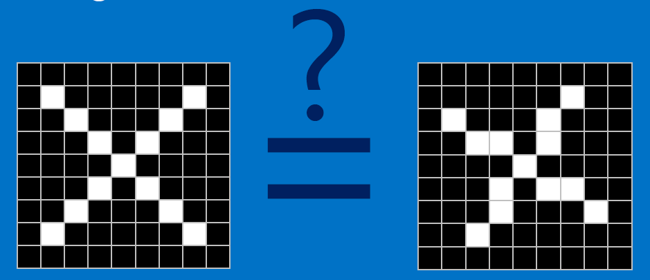
Useful pixels are 1, background pixels are -1:
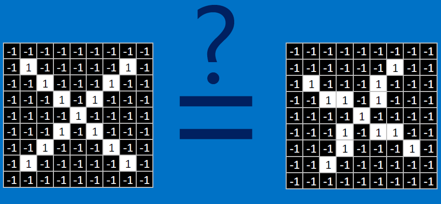
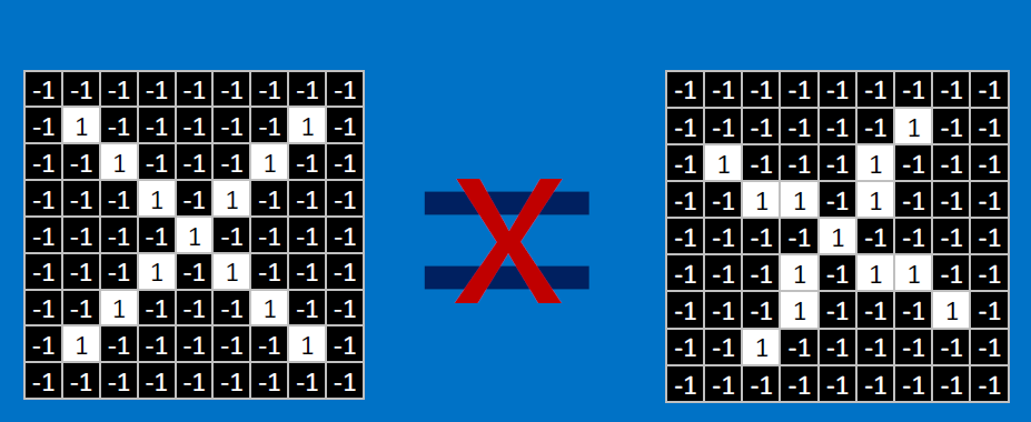
We match SUBREGIONS:
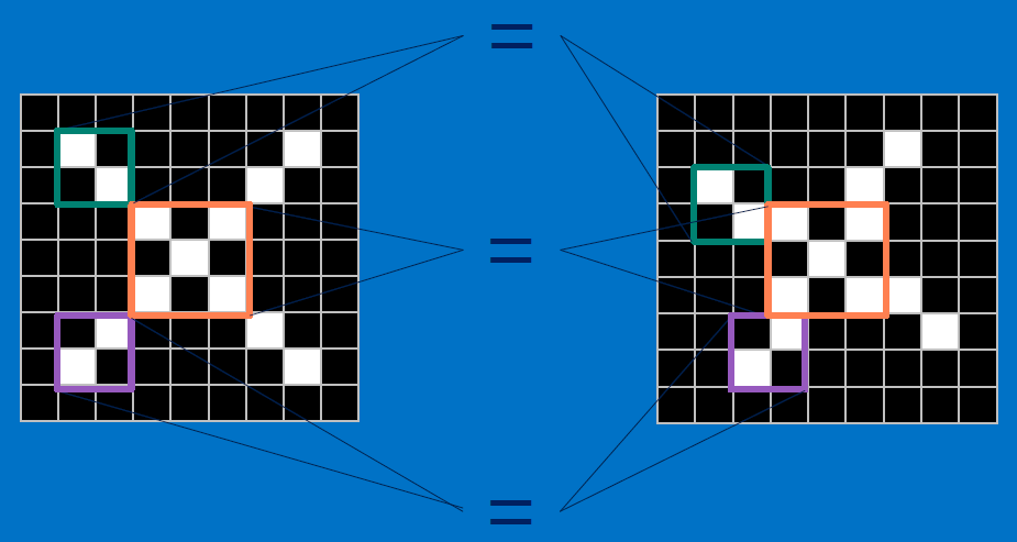
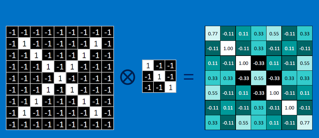
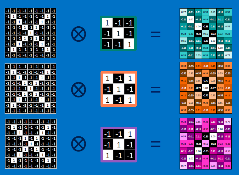
Convolutional neurons that check for these three features:
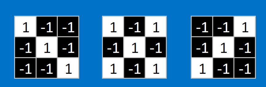
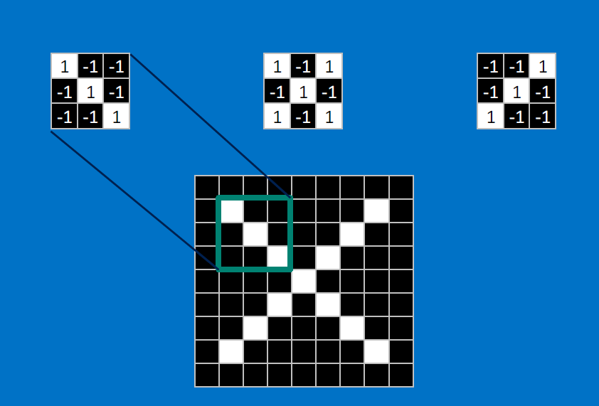
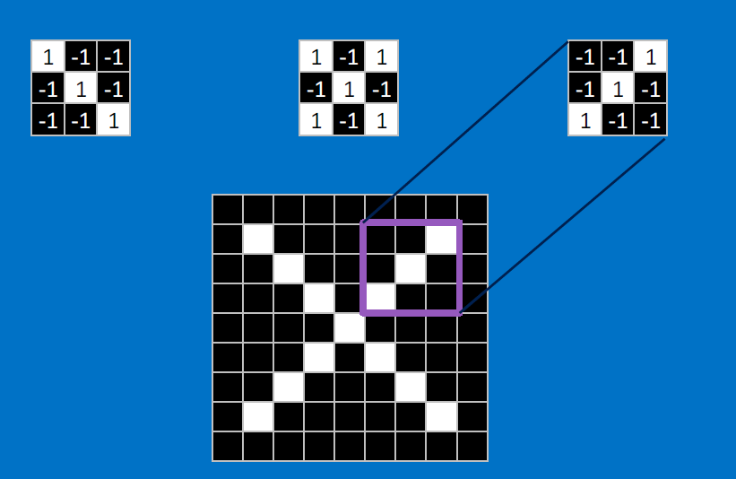
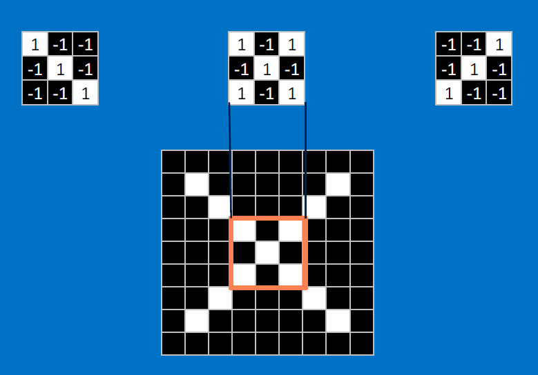
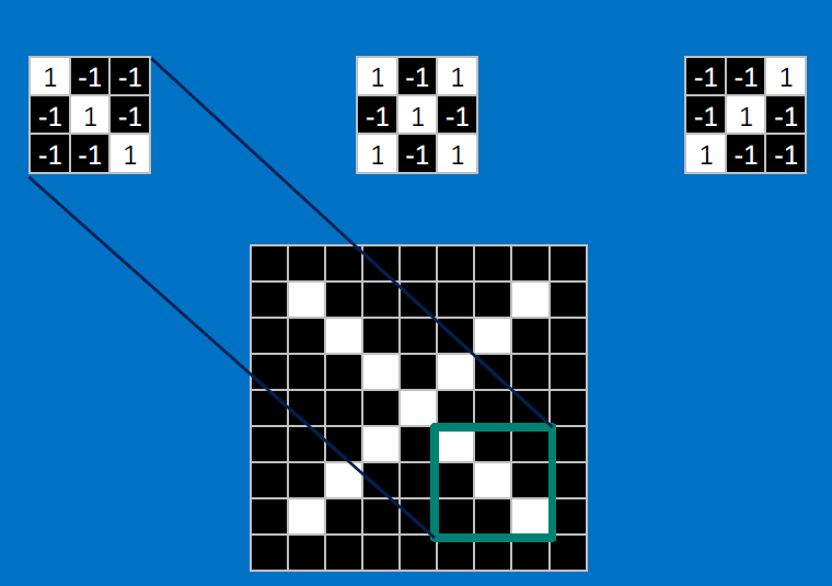
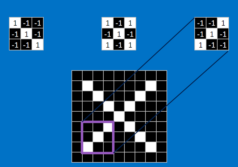
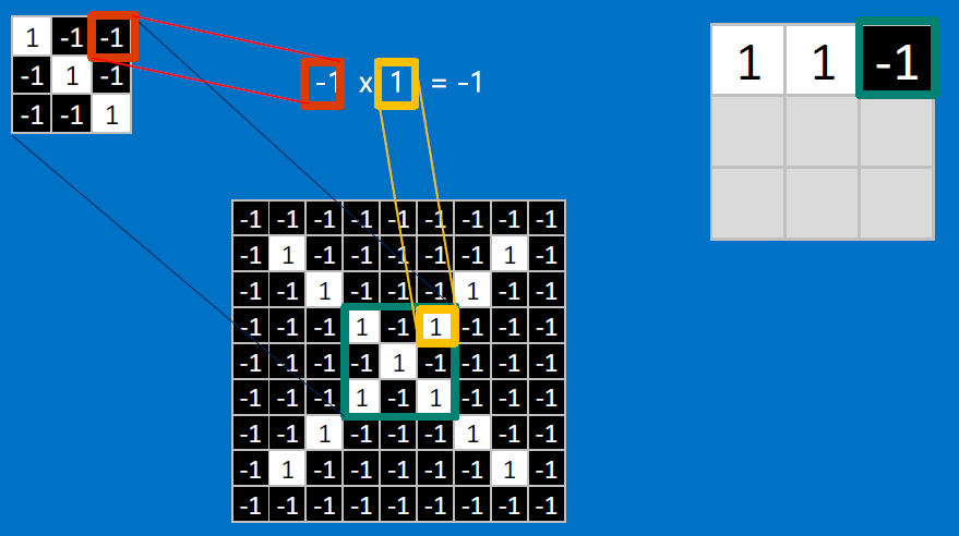
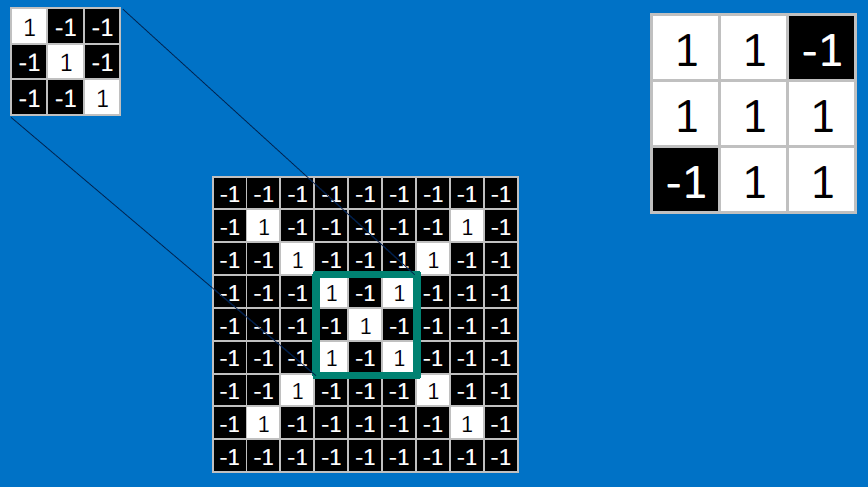
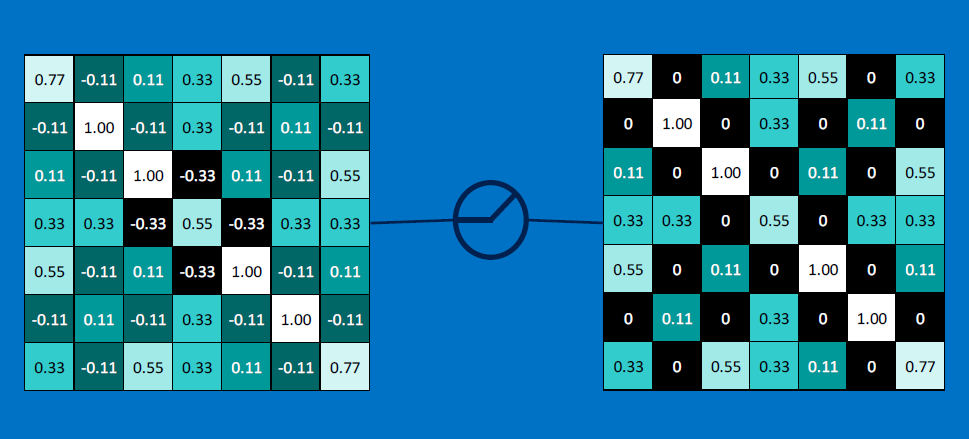
CONVOLVE, ie. do `x_i*w_i`, then average, output a value:
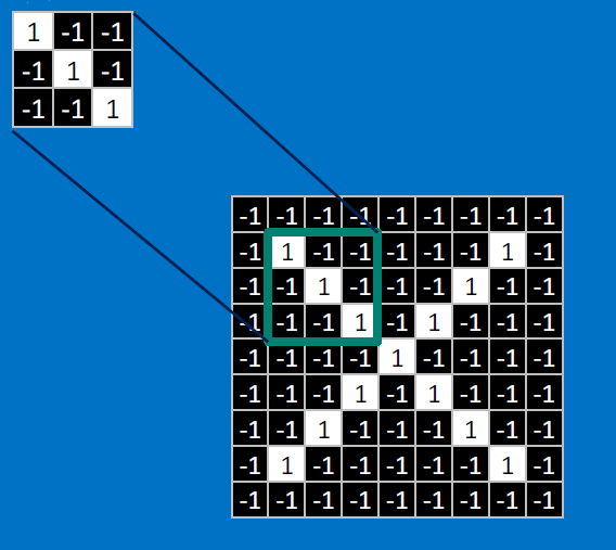
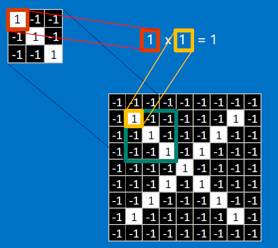
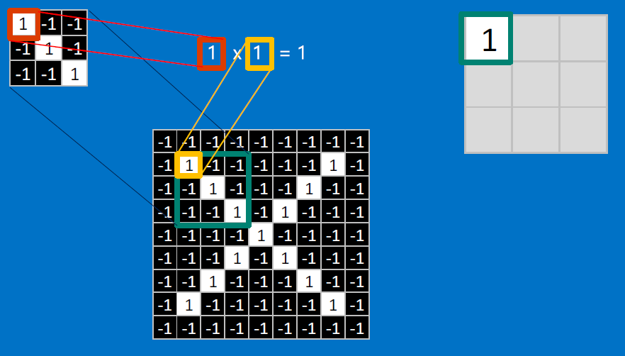
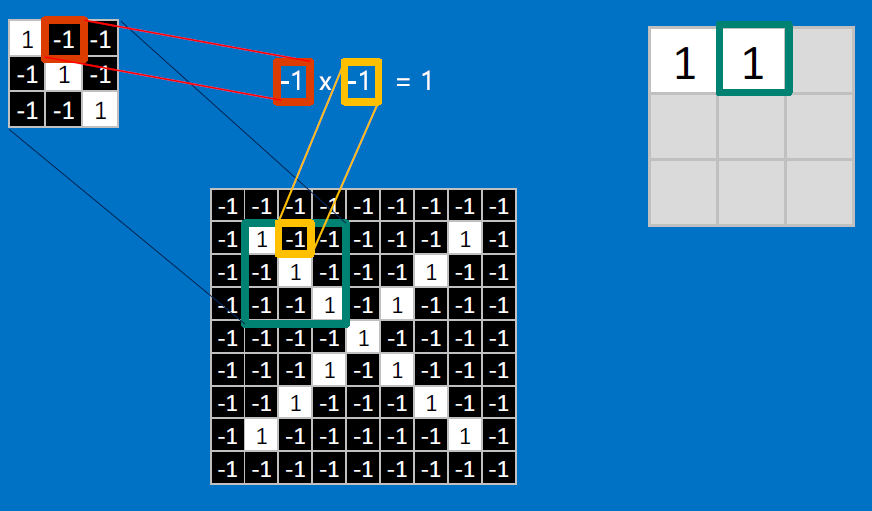
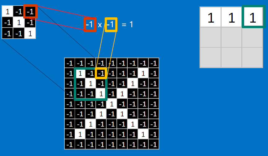
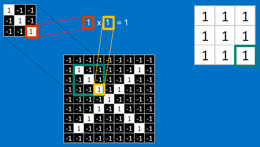
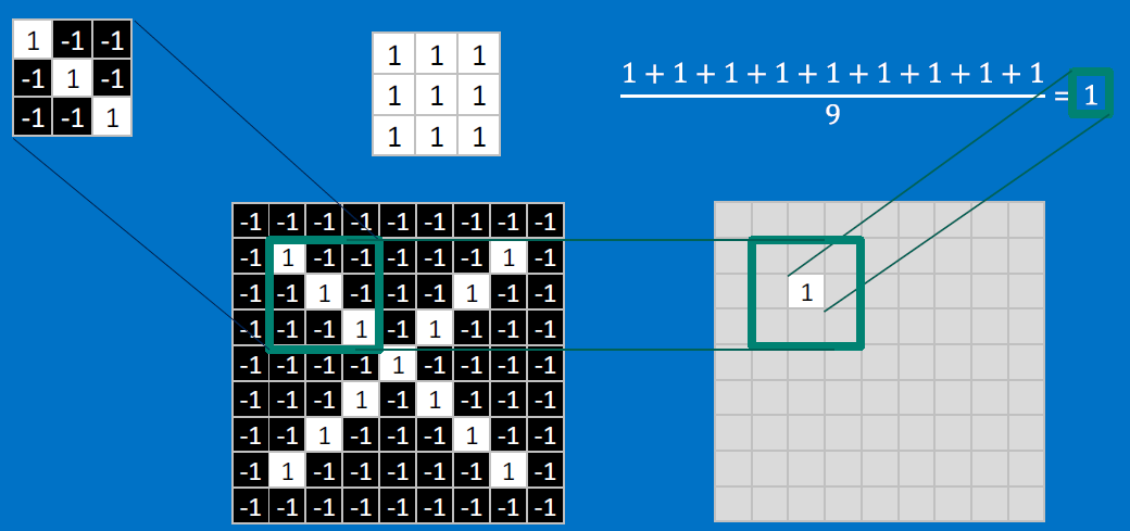
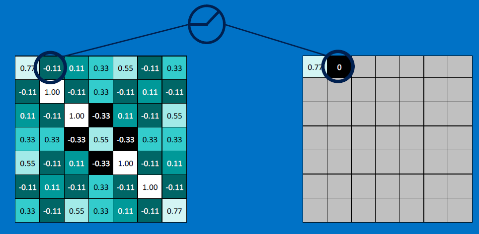
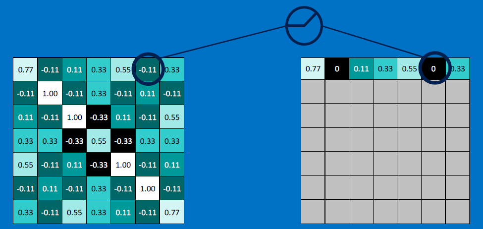
Need to center the kernel at EVERY pixel (except at the edges) and compute a value for that pixel!
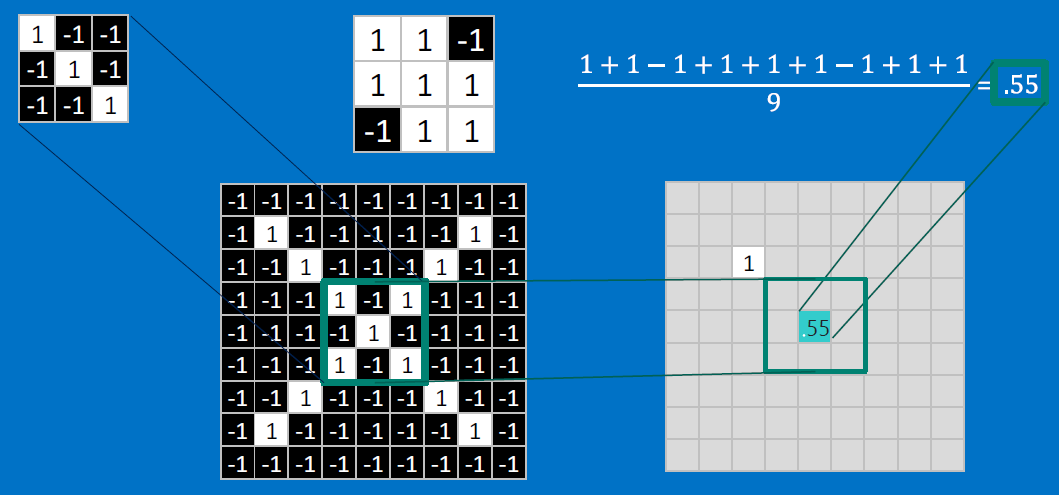
We end up with a 7x7 output grid, just for this (negative slope diagonal) feature:
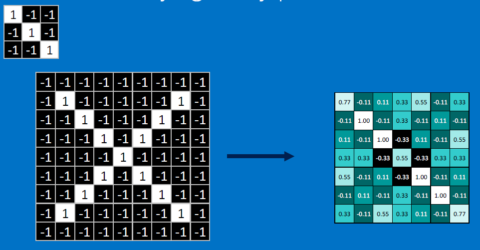
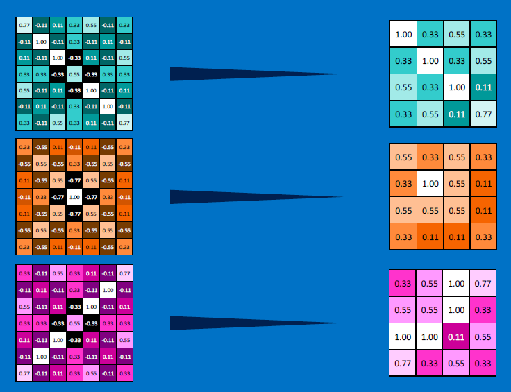
Each neuron (feature detector) produces an output - so a single input image produces a STACK of output images [three in our case, one from each feature detector]:
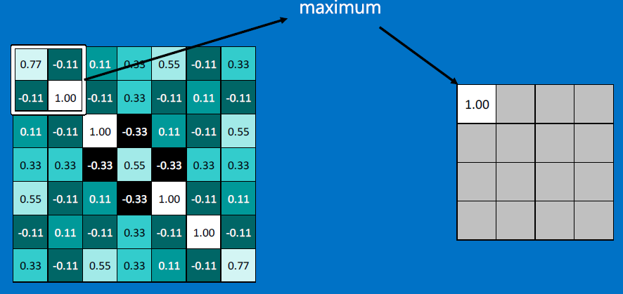
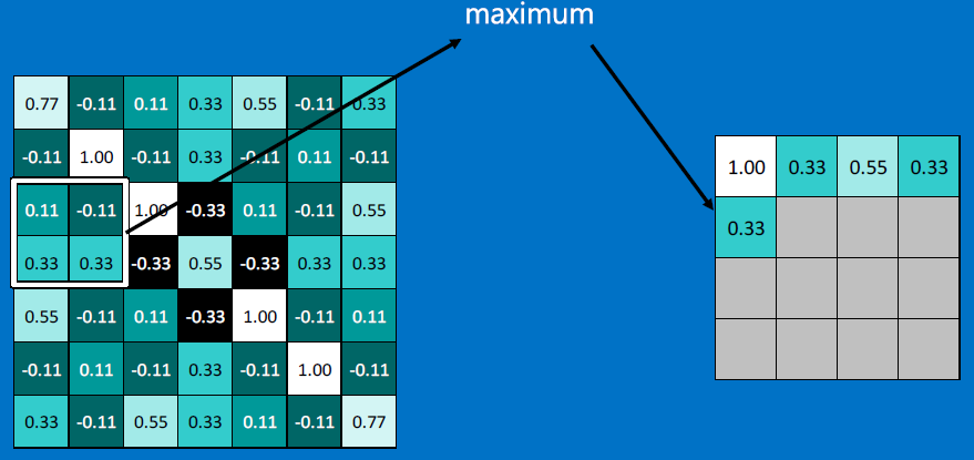
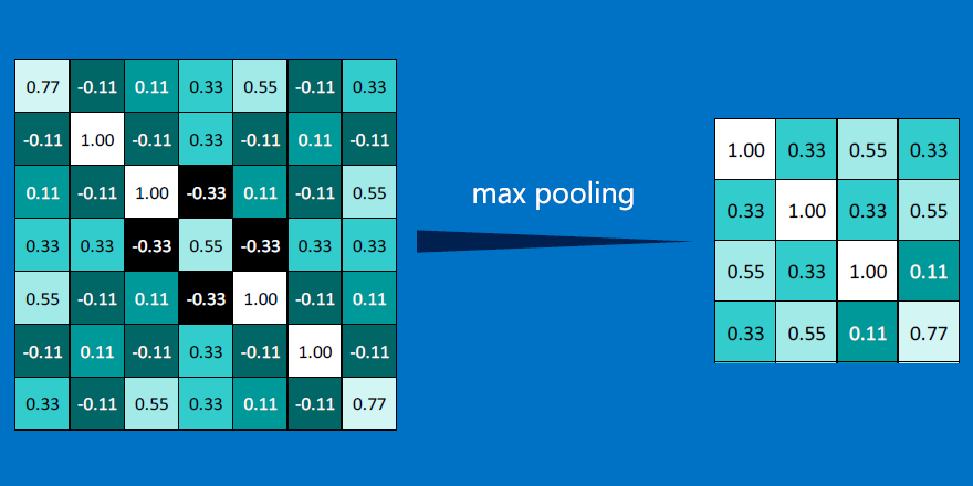
To collapse the outputs, we do 'max pooling' - replace an mxn (eg. 2x2) neighborhood of pixels with a single value, the max of all the m*n pixels.
Next, create a ReLU - rectified linear unit - replace negative values with 0s:
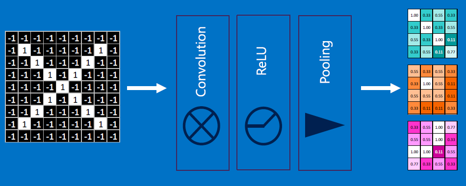
After a single stage of convolution, ReLU, pooling (or eqvt'ly, convolution, pooling, ReLU):
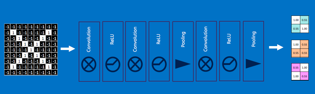
Usually there are multiple stages:
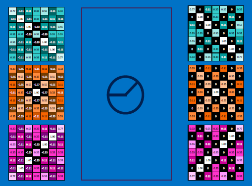
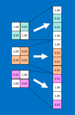
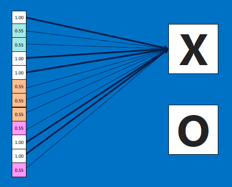
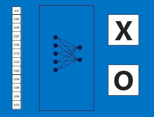
The resulting output values (12 in our case) are equivalent to VOTES: values at #0, #3, #4, #9, #10 contribute to voting for an 'X'; by repeated training with X-like images, which produce high-valued outputs for exactly those values at #0,#3,#4,#9,#10, the RECEIVER of all the 12 values, ie . the 'X' detector, learns to adjust its weights so that those inputs at #0,#3,#4,#9,#10 matter more (get assigned higher weight multipliers) compared to the other inputs such as #1,#2..:
Likewise, if we fed O image detectors kernels' results (also an array of 12 values) to the O receiver, the O receiver would classify it as an O - because the O detector has been separately trained, using several O-like images and O-feature detector neurons!!
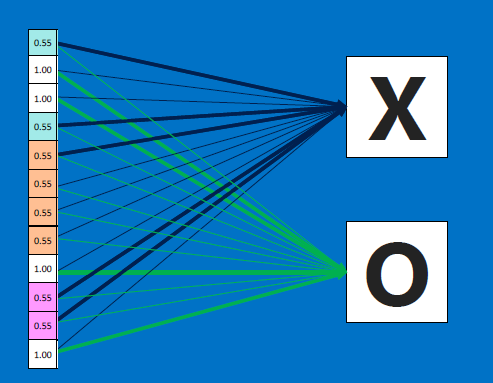
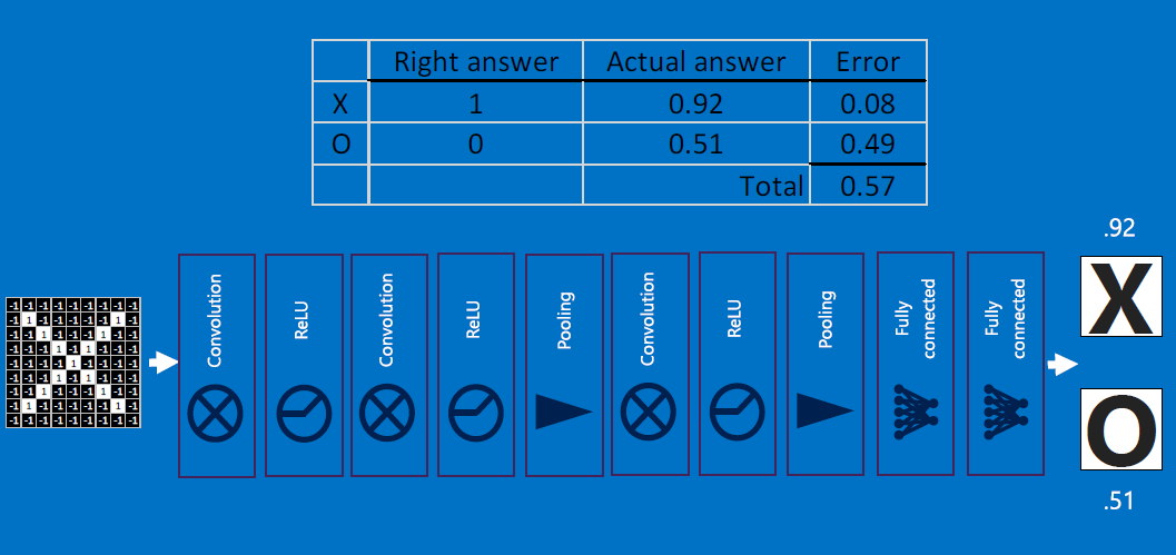
After training, a new ('test') image is fed to BOTH the X feature detector neurons AND to the O feature detector neurons, who outputs are all combined to produce a 12-element array as before. Now we feed that array to both the X-decider neuron and the O-decider neuron:
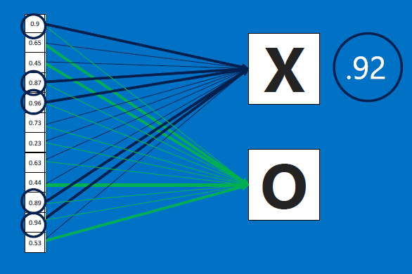
Here's the output for X and O - the results average to 0.91 for X, and 0.52 for O - the NN would therefore classify this as an X:
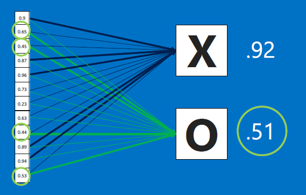
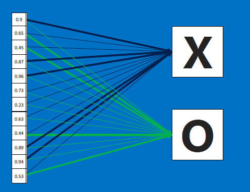
If we feed the network an O-like image instead, the X and O detectors will go to work, and produce an output array where the O features (at #1,#2..) would be higher. So when this array is fed to the X decider and the O decider, we expect the image to be classified as O, eg. because the output probabilities from the X decider and O decider come out to be 0.42 and 0.89.
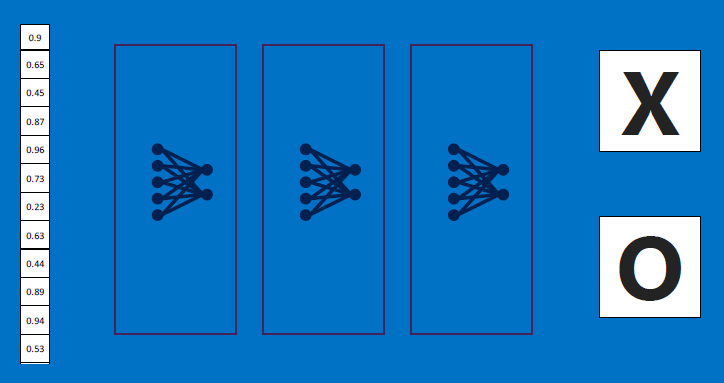
Repeat for each class that needs to be learned: test input => class detectors => outputs => train classifier (at the output layer).
Test input => multiple class detectors => merged results => multiple classifiers (at the output layer) => multiple probabilities => end result.
In summary:
In real world situations, these voting outputs can also be cascaded:
'All together now':
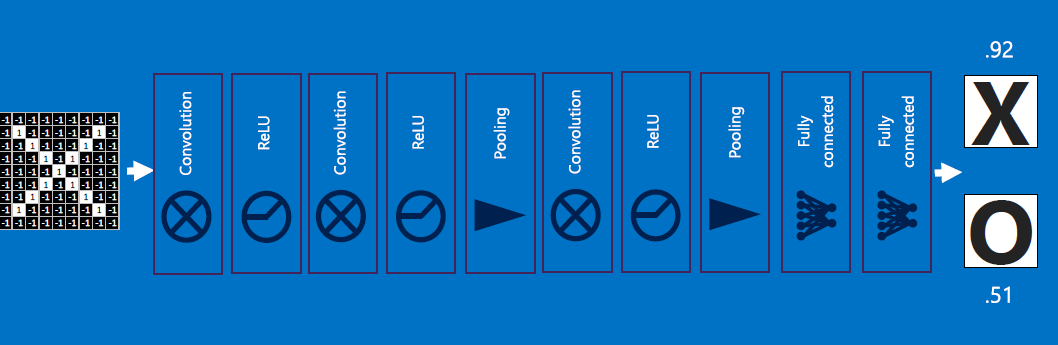
In the above, if we had fed an O-like image instead, the output probability would be higher for O.
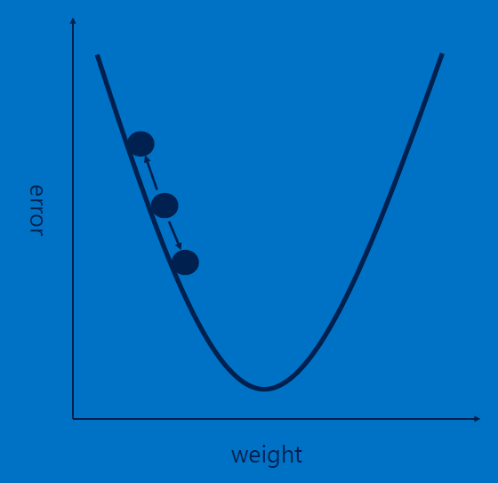
Errors are reduced via backpropagation. Error is computed by taking the absolute differences' sums between expected and observed outputs:
For each feature, each weight (one at a time) is adjustly slightly (+ or -, using the given learning rate) from its current value, with the goal of reducing the error (use the modified weights to re-classify, recompute error, modify weights, reclassify.. iterate till convergence) - this is called backpropagation:
That was a whirlwind tour of the world of CNNs! Now you can start to understand how an NN can detect faces, cars..:
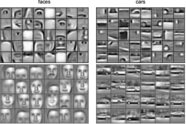
Want to 'learn' more? This 2009 paper has details.
When is a CNN **not** a good choice? Answer: when data is not spatially laid out, ie. scrambling rows and columns of the data would still keep the data intact (like in a relational table) but would totally throw off the convolutional neurons!
NN papers and blogs
Look up papers/blogs by:
- Andrew Ng
- Yann LeCun
- Andrej Karpathy
- Chris Olah
- Brandon Rohrer
Also, this is a VERY comprehensive portal on DNN.
NN libraries, platforms
As you can imagine, there is a wide variety of libraries available.
The following are general purpose ML frameworks:
- TensorFlow - more on this soon
- CAFFE
- Caffe2
- CNTK
- Deeplearning4j
- Keras
- Torch
- Theano
- scikit-learn [used commonly with pandas] - see this and this, for examples
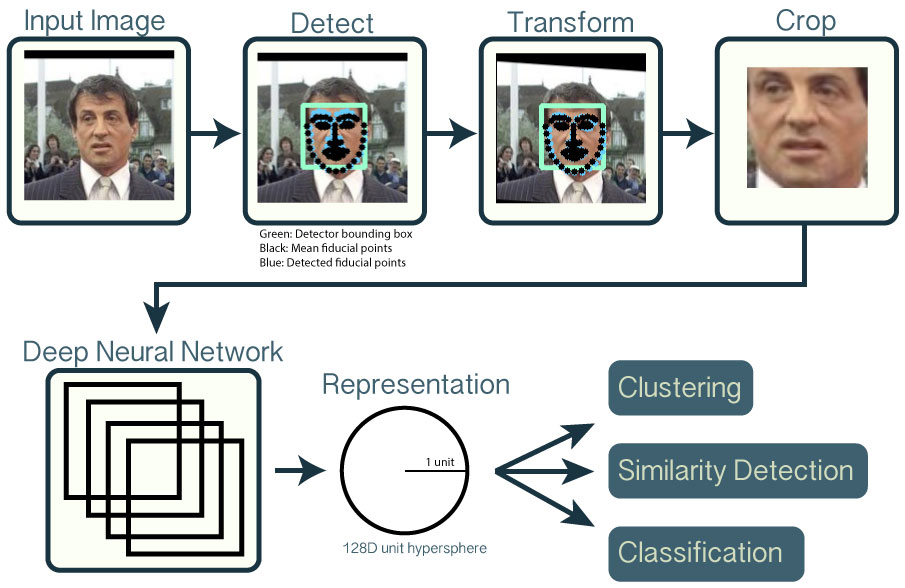
OpenFace is specifically for face detection:
MATLAB offers the following libraries, for developing NN applications: Neural Network Toolbox, Statistics and Machine Learning Toolbox, Parallel Computing Toolbox, Image Processing Toolbox, Computer Vision System Toolbox, Image Acquisition Toolbox, and Signal Processing Toolbox. Likewise, Mathematica offers ML-related functionality.
NN/ML *platforms* are starting to emerge, that package cloud storage, cloud computing and also algorithms/libraries into an out-of-the-box solution for developing and DEPLOYING ML apps! SO MUCH POWER at your fingertips, with ZERO installation and maintenance! Here are the leading ones (the usual suspects):
- https://aws.amazon.com/machine-learning/
- https://azure.microsoft.com/en-us/services/machine-learning/ and https://studio.azureml.net/
- https://cloud.google.com/products/machine-learning/
That's a LOT of tools and platforms! Here is a way for you to dive right in [Lynda.com access is FREE for USC students - log on to Blackboard, look in 'Helpful Resources'].
NN in hardware
The following are GPU-based NN implementations (advantages: massively parallel processing, and possibility of arbitrary speed increases over time just by upgrading hardware!):
In addition, Amazon's AWS now includes cloud-GPU computing!
Facebook plans to open source a GPU-based NN system, making it possible for third-party providers to construct such systems and cloud-enable them (ie. compete with AWS :)).
Like AWS, Algorithmia lets you run NN algorithms on GPU-enabled servers they host. Check out their cool online demos!
And IBM's TrueNorth is a revolutionary, neural-architecture-based chip, meant for general purpose computation in addition to NN implementation.
Last but not least, Google has its own hardware implementation of its NN library [more on this soon].
What is old is new again :)
More things to look up
In no particular order, below are items you need to look up, if you want to get up to speed on the latest developments in NNs. There are developments along two fronts: extensions/mods to the core NN idea, and productizing.
- [aside] math for deep learning
- RNNs, LSTMs [Recurrent Neural Nets (RNNs) are especially good for 'sequence' problems such as speech recognition, language translation, etc.; they are not massively parallelizable the way CNNs can be]
- Temporal Convolution Nets (TCNs) - a good, parallelizable alt to RNNs
- adversarial learning (and GANs)
- 'transfer' learning
- Inceptionism
- Google Quick Draw, AutoDraw, DL portrait morph
- Google's Cloud Vision API: https://cloud.google.com/vision/
- Amazon Rekognition API: https://aws.amazon.com/rekognition/
- Amazon ML Solutions Lab
- Microsoft's Azure ML
- Gluon platform: http://www.businesswire.com/news/home/20171012005742/en/AWS-Microsoft-Announce-Gluon-Making-Deep-Learning
- Capsule Network (CapsNet): https://hackernoon.com/what-is-a-capsnet-or-capsule-network-2bfbe48769cc
What is TensorFlow (TF)?
TensorFlow is an open source offering from Google Brain Team.
Specifically, TensorFlow is a system that processes a dataFLOW graph, where the data that gets passed in and out of each node ("op") in the graph is a TENSOR (typed multi-dim array). Stated another way, it is a dataflow processor where ALL data is in the form of 'tensors' - in other words, tensors flow in and out of ops/nodes that form a (dataflow) graph.
Schematically, every op (node) in a tensorflow graph looks like this:
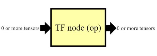
From Google's doc: "TensorFlow uses a dataflow graph to represent your computation in terms of the dependencies between individual operations. This leads to a low-level programming model in which you first define the dataflow graph, then create a TensorFlow session to run parts of the graph across a set of local and remote devices."
Why use TF?
Because CNNs involve pipelined neuron processing, where each neuron (a node in TF) processes arrays of inputs and weights (tensors in TF).
TF makes it possible to express neural networks as graphs (flexible), as opposed to a collection of chained function calls (rigid). The flexibility also allows the nodes to be processed in a variety of ways - in a CPU, GPU, 'TPU', cloud, laptop, mobile device, other hardware...
Setting up/running TF [native, virtualized, cloud]
You can download TF from GitHub via your native Python environment (eg. using pip install), and use it in that environment.
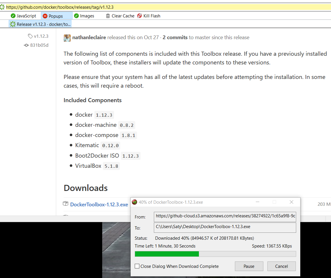
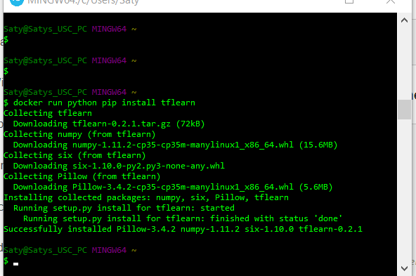
Or you can use Docker! Very simply, Docker is a lightweight alternative to running a VM such as VirtualBox or VMWare. Docker allows for easy downloading and installing of software inside it, using git-style pull requests. For our purposes, we'll need to install Python first, then pull in tensorflow.
Install Docker Toolbox first:
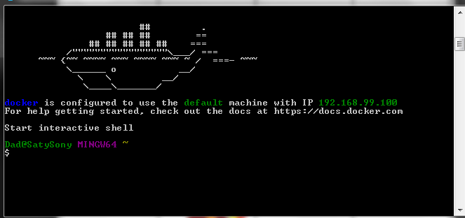
Next, launch a Docker shell (Docker Quickstart Terminal):
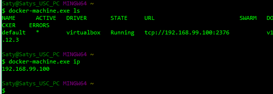
Next, verify that Docker is running properly [note - this screenshot is off a different PC compared to above!]:
Now we can run Hello World :)
Time to install Python, followed by tensorflow:
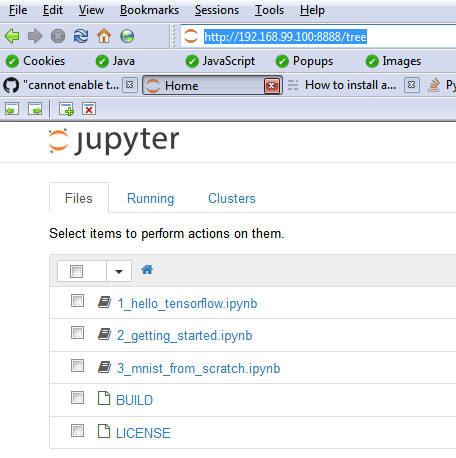
Excellent! Now we can start playing with TensorFlow by visiting localhost:8888 (or http://192.168.99.100:8888) on our browser, and running "literate computing-style" Jupyter notebooks there.
You can even run Jupyter notebooks on the cloud (note - you can't edit using this interface). Eg. here is a pre-loaded example (GitHub can run this, too).
A quick example
Here is an example where we add two "tensors" (arrays of identical length/size) to obtain a resulting "tensor".
Another short example
Here we chain additions:
numpy ("np")
numpy is a popular, capable module that we use with TF.
Mat mult
This is how to multiply two matrices [like we'd do in a CNN!].
A linear regression learner
This short and sweet example shows we can iteratively solve for m and c for a y=mx+c line equation, given pairs of (x,y) data :)
You can use the above as a starting point for more regression experiments - multiple-linear, non-linear..
tensorflow.js
tensorflow.js is a JavaScript port, of the Python-based tensorflow API. Check out the 'demos' part of the link above.
Also, here is a notebook, with JavaScript cells in it containing a TF-based image classifier. Edit the dog pic, change the existing URL to a new one that contains a pic, of one of the 1000 things this network is trained on, see if it can predict what's in your new pic :)
Resources, more info
As you can imagine, we barely scratched the surface! Here are starting points for more exploring:
Also, Magenta (see this page, this one) is an experiment to get NNs to GENERATE art (including music)..
TF is in hardware! Google uses a specialized chip called a 'TPU', and documents TPUs' improved performance compared to GPUs. Here is a pop-sci writeup, and a Google blog post on it.
Here is FBLearner Flow - Facebook's version of TensorFlow :)