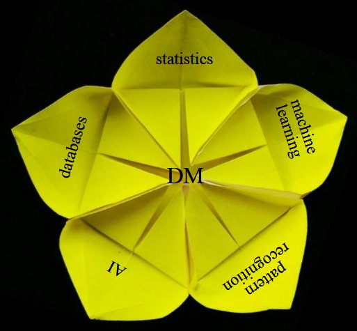
DM is inter-disciplinary
Here is how data mining relates to existing fields:
Data Mining[search(ing) for PATTERNS]"You look at where you're going and where you are and it never makes sense, but then you look back at where you've been and a pattern seems to emerge."
|
Data mining is the science of extracting useful information from large datasets.
At the heart of data mining is the process of discovering RELATIONSHIPS between parts of a dataset.
"Data mining is the analysis of (often large) observational data sets to find unsuspected relationships and to summarize the data in novel ways that are both understandable and useful to the data owner. The relationships and summaries derived through a data mining exercise are often referred to as models or patterns".
The term 'trend' is used to describe patterns that occur or change over time.
How is ML different from DM?
Machine learning is the process of TRAINING an algorithm on an EXISTING dataset in order to have it discover relationships (so as to create a model/pattern/trend), and USING the result to analyze NEW data.
Here is Andrew Ng's 'classic' Stanford course on ML that is hosted at Coursera, which he co-founded [till early 2017, Andrew was with Baidu].
Here is how data mining relates to existing fields:
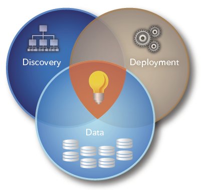
By nature, most data mining is cyclical. Starting with data, mining leads to discovery, which leads to action ("deployment"), which in turn leads to new data - the cycle continues.
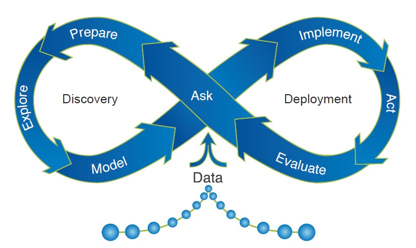
A more nuanced depiction of the cycle:
As you can imagine, data mining is useful in dozens (hundreds!) of fields!! Almost ANY type of data can be mined, and results put to use. Following are typical uses:
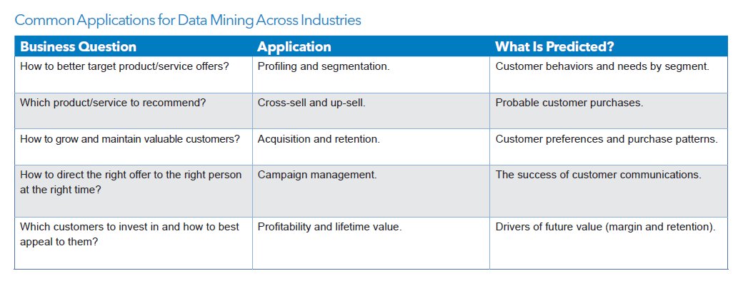

The oil industry is a HEAVY user of data, to predict profitable drilling locations! Look through this, then return to it after we cover a suite of DM algorithms, to make more sense of it :)
As a future exercise, look for many more such case studies, in a variety of 'verticals' (industries/application areas, ie. domains).
Practically all data mining algorithms neatly fit into one of these 4 categories:
We'll look at examples in each category, that will provide you a concrete understanding of the above summarization.
Algorithms can also be classified as being a 'supervised' learning method (where we need to provide categories for, ie. train, using known outcomes), or an 'unsupervised' method (where we provide just the data to the algorithm, leaving it to learn on its own).
Now we can start discussing specific algorithms (where each one belongs to the four categories we just outlined).
Challenge/fun - can each algorithm be talked about, without using any math at all? You get the 'big picture' [a clear, intuitive understanding] that way.. After that, we can look at equations/code for the algorithms, to learn the details (God/the devil *is* in the details :)).
Classification and regression trees (aka decision trees) are machine-learning methods for constructing prediction models from data. The models are obtained by recursively partitioning the data space and fitting a simple prediction model within each partition.
The decision tree algorithm works like this:
Should we play tennis? Depends (on the weather) :)
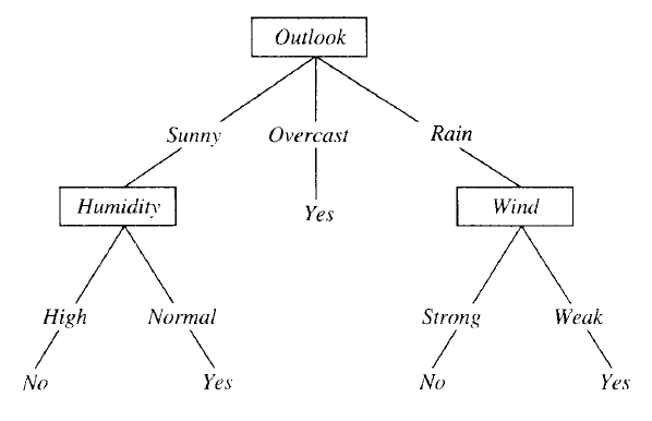
This is a VERY simple algorithm! The entire tree is a disjunction (where the branches are) of conjunctions (that lead down from root to leaves).
If the outcome (dependent, or 'target' or 'response' variable) consists of classes (ie. it is 'categorical'), the tree we build is called a classification tree. On the other hand if the target variable is continuous (a numerical quantity), we build a regression tree. Numerical quantities can be ordered, so such data is called 'ordinal'; categories are names, they provide 'nominal' data. Given that, nominal data results in classification trees, and ordinal data results in regression trees.
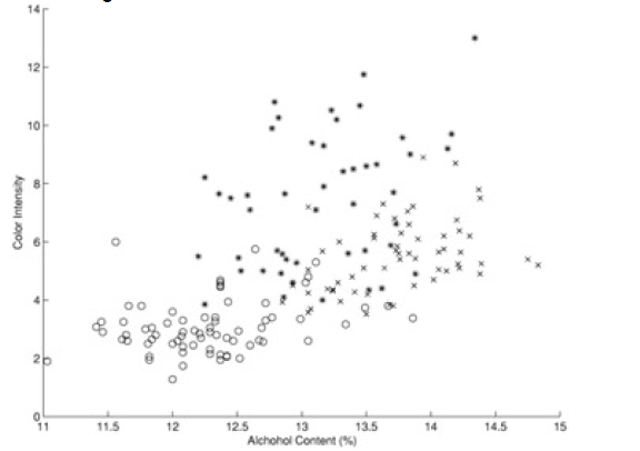
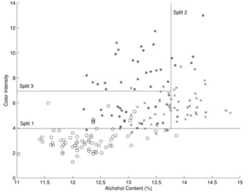
Here is another example (from 'Principles of Data Mining' by David Hand et. al.). Shown is a 'scatter plot' of a set of wines - color intensity vs alcohol content:
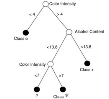
The classification tree for the above data is this:
When we superpose the 'decision boundaries' from the classification tree on to the data, we see this:
A sample regression tree is shown below - note that the predictions at the leaves are numerical (not categorical):
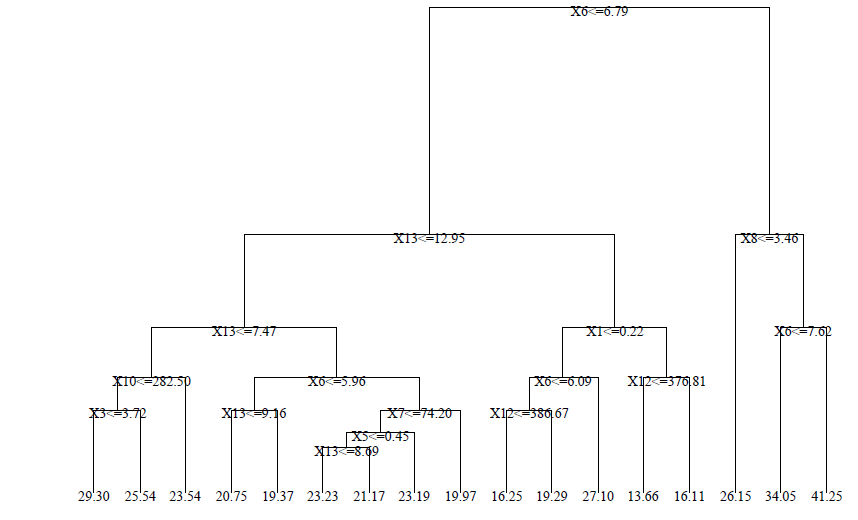
Note - algorithms that create classification trees and regression trees are referred to as CART algorithms (guess what CART stands for :)).
This algorithm creates 'k' number of "clusters" (sets, groups, aggregates..) from the input data, using some measure of closeness (items in a cluster are closer to each other than any other item in any other cluster). This is an example of an unsupervised algorithm - we don't need to provide training/sample clusters, the algorithm comes up with them on its own.
If each item in our (un-clustered) dataset has 'n' attributes, it is eqvt to a point in n-dimensional space (eg. n can be 120, for Amazon!). We are now looking to form clusters in n-D space!
Approach: start with 'n' random locations ('centroids') in/near the dataset; assign each input point (our data) to the closest centroid; compute new centroids (from our data); iterate (till convergence is reached).
Here is a use case for doing clustering:
Again, very simple to understand/code!
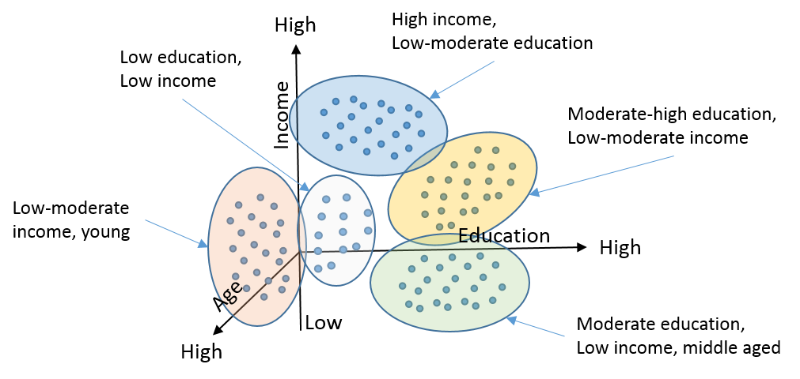
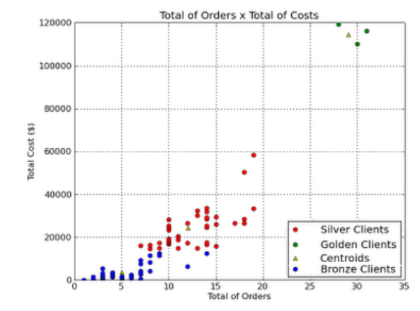
Another example - here, we classify clients of a company, into 3 categories, based on how many orders they placed, and what the orders cost:
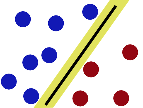
An SVM always partitions data (classifies) them into TWO sets - uses a 'slicing' hyperplane (multi-dimensional equivalent of a line), not a decision tree.
The hyperplane maximizes the gap on either side (between itself and features on either side). This is to minimize chances of mis-classifying new data.
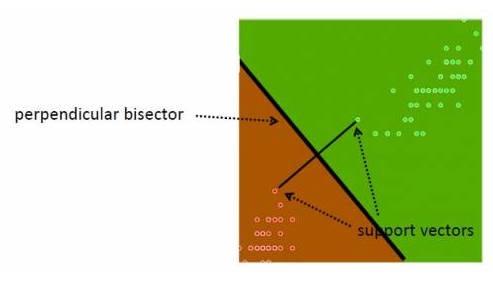
On either side, the equidistant data points closest to the hyperplane are the 'support vectors' (note that there can be several of these, eg. 3 on one side, 2 on the other). Special case - if there is a single support (closest point) on either side, in 2D, the separator is the perpendicular bisector of the line segment joining the supports; if not, the separating line/plane/hyperplane needs to be calculated by finding two parallel hyperplanes with no data in between them, and maximizing their gap. The goal is to achieve "margin maximization".
How do we know that a support data point is indeed a support vector? If we move the data point and therefore the boundary moves, that is a support vector :) In other words, non-support data can be moved around a bit, that will not change the boundary (unless the movement brings it to be inside the current margin).
Note - in our simplistic setup, we make two assumptions: that our two classes of data are indeed separable (not inter-mingled), and that they are linearly separable. FYI, it is possible to create SVMs even if both the assumptions aren't true.
Here's some geek humor for ya:
Looking for hidden relationships in large datasets is known as association analysis or association rule learning.
The A priori algorithm comes up with association rules (relationships between existing data, as mentioned above). Here is an example: outputting "items purchased together" (aka 'itemsets'), eg. chip, dip, soda, from grocery transaction records.
Inputs: data, size of the desired itemsets (eg. 2, 3, 4..), the support (number of times the itemset occurs, divided by the total # of data items) and the confidence (conditional probability of an item being in a datum, given another item in the datum).
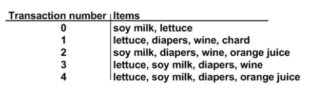
In the above, support for {soy milk,diapers} is 3/5 [again, 'support' is the fraction of "our" occurrence).
Also in the above, the confidence for {diapers} -> {wine} is support({diapers,wine})/support({diapers}), which is 3/5 over 4/5, which is 0.75. We don't need to divide by totals, they cancel out anyway - so 'confidence' of "if they buy diapers, they will also buy wine" is simply "occurrences of diapers+wine, over occurrences of diapers+anything[including wine]", which for us is 3/4. Generalizing, 75% of the time, purchasing diapers seems to lead to purchasing wine as well. Note that in the above, the confidence of {diapers->soy milk} is also 0.75 (again, 3/4).
What is specified to the algorithm as input, is a (support,confidence) pair, and the algorithm outputs all matching associations - we would then make appropriate use of the results (eg. co-locate associated items in a store, put up related ads in the search page, print out discount coupons for associated products while the customer is paying their bill nearby, etc.).
Below is another 'shopping basket' example, with products in columns, customers in rows.
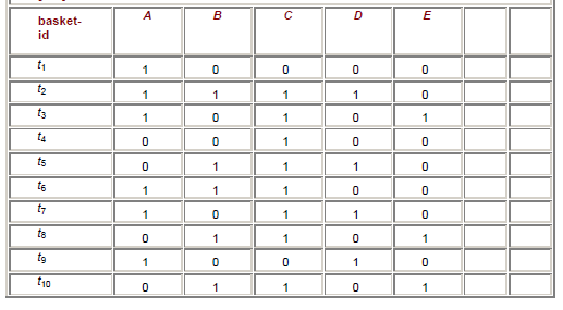
If we set a frequency (ie support) threshold of 0.4 and confidence of 0.5, we can see that the matching items are {A}, {B}, {C}, {D}, {A,C}, {B,C} (each of these occur >=4 times). We can see that {A,C} has an accuracy (ie. confidence) of 4/6=2/3 [occurences-of-AC/occurences-of-A], and {B,C} has an accuracy of 5/5=1 [EVERY time B is purchased, C is also purchased!].
Summary: given a basket (set of itemsets), we can look for associations between itemsetA and itemsetB, given:
So if our five inputs listed above are (2,1,0.4,0.4,0.5) in the above basket example, the outputs would be (A,C) and (B,C), which means we'd consider co-locating or co-marketing (A,C) and also (B,C) - this is the actionable result we get, from mining the basket data.
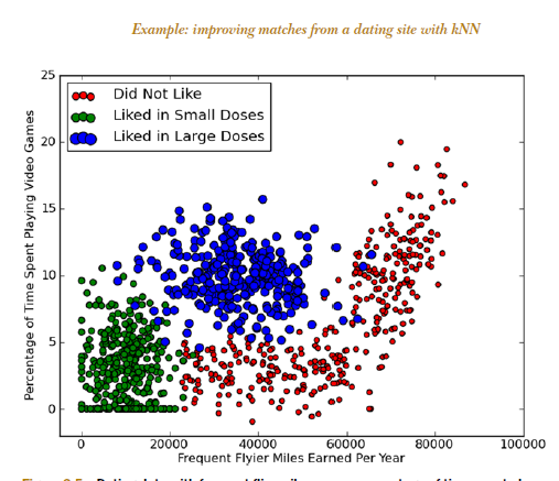
kNN (k Nearest Neighbors) algorithm picks 'k' neartest neighbors, closest to our unclassified (new) point, considers the 'k' neighbors' types (classes), and attempts to classify the unlabeled point using the neighbors' type data - majority wins (the new point's type will be the type of the majority of its 'k' neighbors).
Here is an example of 'loan defaulting' prediction. With k=3, and a new point of (42,142000), our neighbors have targets of Non Default, Non Default, Default - so we assign 'Non Default' as our target.
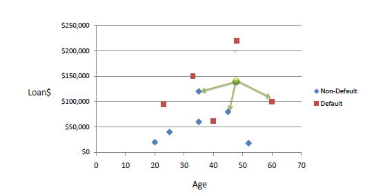
Note that if k=1, we assign as our target, that of our closest point.
Also, to eliminate excessive influence of large numerical values, we usually normalize our data so that all values are 0..1.
kNN is a 'lazy learner' - just stores input data, uses it only when classifying an unlabeled (new) input. VERY easy to understand, and implement!
In some situations (where it is meaningful to do so), it is helpful to separate items in a dataset into hierarchical clusters (clusters of clusters of..). There are two ways to look at this - as the merging of smaller clusters into bigger superclusters, or dividing of larger clusters into finer scale ones.
Below is a dataset that plots, for Yellowstone National Park, the waiting time between geyser eruptions, and length of eruptions. The data points are numbered, just to be able to identify them in our cluster diagram.
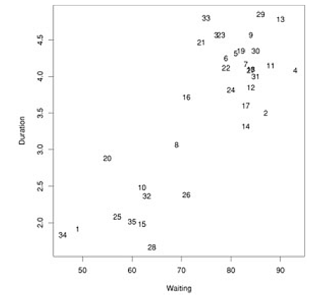
Given this data, we run a hierarchical clustering algorithm, whose output is a 'dendogram' (tree-like structure) that shows the merging of clusters:
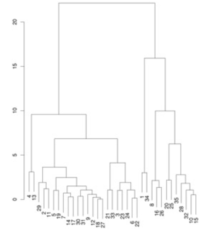
How do we decide what to merge? A popular strategy - pick clusters that lead to the smallest increase in sum of squared distances (in the above diagram, that is what the vertical bar lengths signify). The dendogram shows that we need to start by merging #18 and #27, which we can verify by looking at the scatter plot (those points almost coincide!).
What is the difference between classification and clustering? Aren't they the same?
Classification algorithms (when used as learning algorithms) have one ultimate purpose: given a piece of new data, to place it into one of several pre-exising, LABELED "buckets" - these labels could be just names/nonimal (eg. ShortPerson, Yes, OakTree..) or value ranges/ordinal (eg. 2.5-3.9, 100,000-250,000)..
Clustering algorithms on the other hand (again, when used as learning algorithms) take a new piece of data, and place it into a pre-existing group - these groups are UN-LABELED, ie. don't have names or ranges.
Also, in parameter (feature/attribute) space, each cluster would be distinct from all other clusters, by definition; with classification, just 'gaps' don't need to exist.
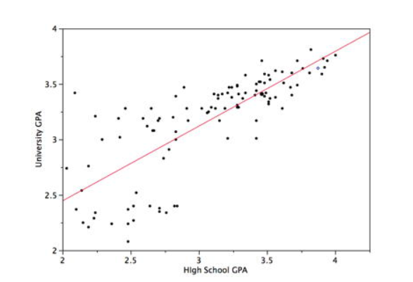
This (mining) technique is straight out of statistics - given a set of training pairs for a feature x and outcome y, fit the best line describing the relationship between x,y. The line describes the relationship/pattern.
Given that we have Yi which depends on Xi1,Xi2,Xi3...Xip [i is the sample index, 1,2,3..p are the variable indices (dimensions)], model the dependency relationship as Yi=f(Xi)+εi where f is the unknown function (that we seek), and ε is the error with mean=0.
Here is an example:
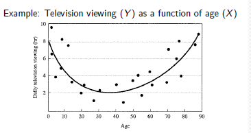
Here we fit a higher order polynomial equation (parabola, ie. ax2+bx+c) to the observed data:
Here we need to fit a higher order, non-linear surface (ie. non-planar) to the observed data:
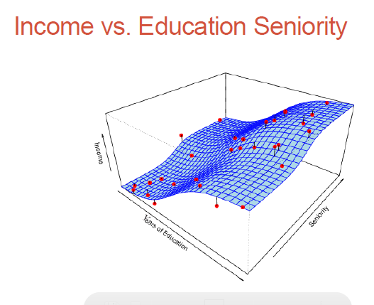
...
Parametric methods (eg. regression analysis which we just looked at) involve parameter estimation (regression coefficients).
Non-parametric methods - no assumptions on what our surface (the dependent variable) would look like; we would need much more data to do the surface fitting, but we don't need the surface to be parameter-based!
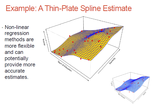
While non-parametric models might be better suited to certain data distributions, they could lead to a poor estimate as well (if there is over-fit)..

Logistic regression is a classification (usually binary) algorithm:
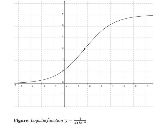
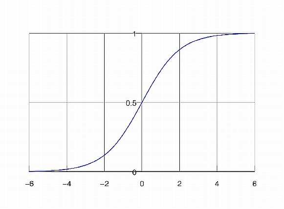
Result (the whole point of doing the three steps above) - we are transforming a continuous, regression-derived value (which can be arbitrarily large or small) into a 0..1 value, which in turn we transform into a binary class (eg. yes or no) [similar to using an SVM or creating two clusters via k Means]. Note that if we use the simpler form of the logistic equation (a=b=c=1), we'd need to transform our regression results to a 0-centered distribution before using the logistic equation - this is because 1/(1+exp(-x)) is 0.5, when x=0.
Uses?
The 'naïve' Bayes algorithm is a probability-based, supervised, classifier algorithm (given a datum with x1,x2,x3..xn features, classify it to be one of 1,2,3...k classes).
The algorithm is so called because of its strong ('naïve') assumption: each of the x1 ..xn features are statistically independent of each other ["class conditional independence"] - eg. a fruit is an apple if it is red, round and ~4 in. dia.
Other names for this algorithm: simple Bayes, independence Bayes, idiot Bayes (!).
For each training feature set, probabilities are assigned for each possible outcome (class). Given a new feature, the algorithm outputs a classification corresponding to the max of the most probable value of each class (which the algorithm calculates, using the 'maximum a posteriori', or 'MAP' decision rule).
Here is an example (from http://www.statsoft.com/textbook/naive-bayes-classifier).
Given the following distribution of 20 red and 40 green balls (ie. 60 samples, 2 classes [green,red]), how to classify the new [white] one ('X')?
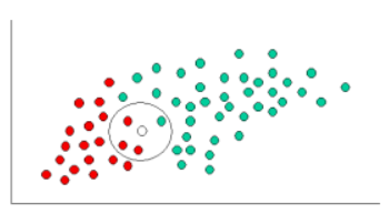
PRIOR probability of X being green or red:
Given the neighborhood around X, probability (LIKELIHOOD) of X being green, X being red:
POSTERIOR probability of X being green, X being red [posterior probability = prior probability modified by likelihood]:
Classify, using the max of the two posterior probabilities above: X is classified as 'red'.
EM is a rather 'magical' algorithm that can solve for a Catch-22 (circular reference) set of values!
Imagine we have a statistical model that has some parameters, regular variables, and some 'latent' (hidden) variables. The model can operate on new data (predict/classify), given training data. Sounds like a straightforward DM algorithm (eg. k means clustering), except that it is not!
We do not know the values for the parameters or latent variables! We DO have observed/collected data [for the regular variables], which the model should be able to act on.
The algorithm works as follows:
As counter-intuitive as it sounds, this does work!
Here is another explanation, from a StackOverflow post:
There's a chicken-and-egg problem in that to solve for your model parameters you need to know the distribution of your unobserved data; but the distribution of your unobserved data is a function of your model parameters.
E-M tries to get around this by iteratively guessing a distribution for the unobserved data, then estimating the model parameters by maximizing something that is a lower bound on the actual likelihood function, and repeating until convergence:
This clip shows an example of EM being used to compute clustering on a dataset. Note how each data point's probability of belong to each cluster, gets updated on account of iterating.
EM is an example of a family of maximum likelihood estimator algorithms - others include gradient descent, and conjugate gradient algorithms.
One more example: EM clustering of Yellowstone's Old Faithful eruption data:
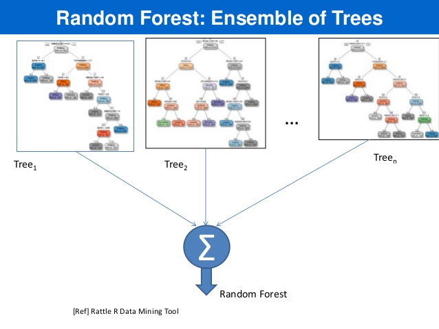
What if we used a training dataset to train several different algorithms - eg. decision tree, kNN, neural net(s)..? You'll most likely get (slightly!) different results for target prediction.
We could use a voting scheme, and use the result as the overall output. Eg. for a yes/no classification, we'd return a 'yes' ('no') if we got a 'yes' ('no') majority.
This method of combining learners' results is called 'boosting', and resulting combo learner is called an 'ensemble learner'. Why do this? "Wisdom of the crowds" :) We do this to minimize/eliminate variances between the learners.
FYI - 'AdaBoost' (Adaptive Boosting) is an algorithm for doing ensemble learning - here, the individual learners' weights are iteratively and adaptively tweaked so as too minimize overall classification errors [starting from a larger number of features used by participating learners to predict outcomes, the iterative training steps select only those features known to improve the predictive power of the overall model].
FYI - 'Bagging' (bootstrap aggregating) is a data-conditioning-related ensemble algorithm (where we employ 'bootstrap resampling' of data - divide the data into smaller subsets, use all the subsets for training different 'variations' of a model, use all the resulting models to predict outcomes, transform these into a single 'ensemble' outcome).
RandomForest(TM) is an *ensemble* method where we: