Lab 2

Scopes and Signals

Introduction

This lab assignment has three purposes:

• Learn how to use the oscilloscope to observe and analyze signals. An important aspect of this is learning how to set up the oscilloscope triggering so both periodic and non-periodic signals can be clearly seen.
• Use the oscilloscope to measure the time it takes for digital signals to propagate through gates.
• Use multiple power supplies and the DMM to determine the logic threshold of a gate.

Due to the number of students in the lab session there may not be sufficient oscilloscopes for each student to work individually. In this case you can work with a partner as a team of two. Teams of three should not be necessary and will only be allowed with the instructor's approval. If you are working with a partner, everyone on the team should take turns working with the oscilloscope and doing the breadboard wiring so all team members learn how to do this. Don't just sit there and watch someone else do the work. In future labs you will have to do the work all by yourself and this is your chance to learn how to do it.

Important: All students are required to submit their own copy of the Lab 2 answers by the due date even if you are working with a partner. A paper work sheet is provided in VHE 205 for recording answers to the questions below that will be turned in using the Lab2_Answers.txt file. To download a copy of the work sheet, click here.

Part 1: Using an Oscilloscope

An oscilloscope is used to show a graph of one or more signals as they change with time. The scope plots a picture of the signal showing the signal's:

• Voltage level along the vertical axis, and
• Time along the horizontal axis

By displaying multiple signals on the same plot, it's possible to see how they are interacting with each other. The scopes in VHE 205 are capable of displaying signals from four signals (channels 1-4) at the same time on the display.

Note: The oscilloscopes in VHE 205 were made by Agilent, but the company is now called Keysight. Some of the pictures of the scope screens many show the Agilent name, while others may say Keysight, but the only difference is in the name. If the name on your scope screen doesn't match the one in this web page, just ignore the mismatch.

To get started follow the steps below.

1. Turn on the oscilloscope by pressing the white button in the lower left of the front panel and wait for it to go through a bunch of self tests. In less than a minute it should be ready to go.
2. Press the "Default Setup" button in the upper right portion of the front panel.
3. After it says on the screen that the default setup has been restored, press the "Back" button in the lower left corner. This should restore the scope to the default settings in case someone has altered them. You should see a screen like this.

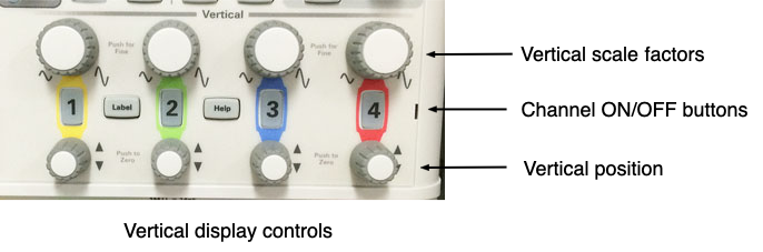
Notice the grid lines on the screen. There are eight vertical grid spaces (a.k.a. "divisions") and ten horizontal "divisions". These can be used in conjunction with the vertical and horizontal scale factors to measure the voltages and timing of signals. The first two numbers to look for are the scale factors for the vertical and horizontal axis. The vertical scale factor is shown in the upper left corner of the screen, and the horizontal scale factor is also along top about 2/3 of the way to the right side.

Note: Each of the four channels can have a different vertical scale factor and these are shown along the upper left of the screen (i.e. channel 1 can be displayed with each division representing 1V while channel 2 is displayed 5V per division). In the default settings, only channel 1 (yellow) is turned on, and the display shows that the vertical scale factor is "5.00V". This means that each of the grid lines represents 5 volts of signal level. The horizontal scale factor is set to "100μs" meaning that the signal is plotted with each horizontal grid space representing 100 microseconds of time. We'll be using the grid lines and the vertical and horizontal scale factors to make voltage and time measurements on signals.

Since there is no input signal connected to channel 1, the plot or "trace" for channel 1 is just a horizontal line across the screen. Look at the left side of the screen where the horizontal line ends. You should see a small "Ground" symbol there aligned with the line. This is how the scope shows you where the Ground or 0 Volt level is displayed on the screen. Since there is no input signal on channel 1, the whole display for that channel is at the ground level.

The position of the trace can be adjusted with the small knob just below the illuminated "1" in the Vertical section of the front panel. Try rotating that knob back and forth and observe how the trace, and the ground indicator, move up and down on the screen. The position knobs for the four channels are used to spread the four traces out on the screen so you can see them.

Now let's look at some signals.

1. Open up the storage compartment on the top of the scope and remove the scope probe that has the yellow markers on the cable. The probes should have colored bands on them, either yellow or green. These are there so when you are using multiple probes you can easily see which probe is associated with each signal trace on the screen.
2. Insert the probe's connector onto the metal BNC connector for channel one. To make proper contact, the connector needs to be pushed onto the scope's connector fully and then rotated clockwise to lock it in place. You'll know it's locked in place if you can't pull it off (with a gentle pull) without first rotating it counter-clockwise.
3. At the other end of the cable, the probe has a metal hook at the tip that is exposed by pulling back on the plastic body of the probe. At the lower edge of the scope, hook the probe tip onto the metal tab that says "Probe Comp" just right of the USB port.

   

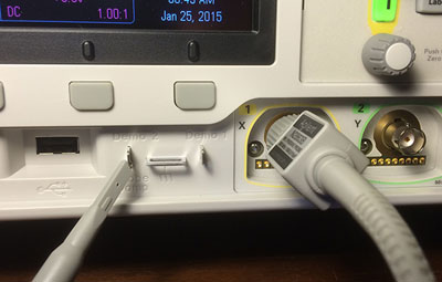
Note 1: The "Probe Comp" metal tab is only used for testing and calibrating the scope. We don't use it for any of our normal measurements. This is probably the only time this semester that you will be attaching the probe to it.

Note 2: The black ground clip on the probe does not have to be connected to a ground point when the probe is attached to the Prop Comp test point. In all other situations the ground lead must be connected to the circuit ground in order work.

You should now see two yellow lines going across the screen about a half a grid spacing apart. To get a better view of the signal we need to change the vertical scale factor to make the signal bigger on the screen.

4. In the Vertical section of the front panel, just above the illuminated "1", the large knob is the vertical scale adjustment. There is one for each channel. Rotate the one for channel 1 a couple of clicks to change the vertical scale factor to 1.0 volts/division (shown at the top left of the display) and this will move the two yellow lines further apart.

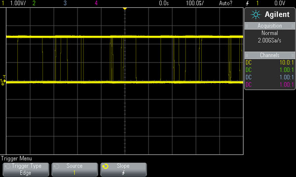
You should be able to see a lot of vertical lines running around on the screen between the two horizontal lines. The display should look something like this.

The next step is to get the display to sit still so we can see what it looks like. To do this we need to set up the triggering on the scope. On an oscilloscope, "triggering" means the set of conditions that cause the scope to start drawing a picture of the signals present on its input channels.

Understanding how triggering works and setting up the triggering conditions is probably the most important aspect of making a scope into a useful diagnostic tool.

The scope can be set to trigger when the input signal meets a set of conditions and it will then display the signals on all the channels that occurred before and after that time. It will then wait until the conditions are met again, and then display the signal again. With periodic signals this gives you stable display of the signals since each time they are drawn on the screen they are in the same position. When the scope doesn't know what to trigger on (like now), it just shows a running (live-stream) display of the incoming signal which usually results in the plot of the signal dancing around on the screen. While you are seeing the signal, it probably won't be stable on the screen and it will be difficult to analyze. When the triggering has been adjusted properly a stable display will be shown and you can get a clear look at the shape of the signal.

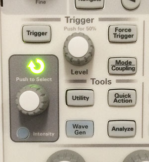
5. In the Trigger portion of the front panel, press the "Trigger" button and the Trigger Menu will appear at the bottom of the screen. Pressing the button below one of the options will bring up a list of all the possible settings for that option. Note that the one pressed will also have a green circle with an arrow on it. This indicates that the setting can be adjusted using the knob just below the "Trigger" button.

   

   Trigger Type

   Determines what type of signal to trigger on. Pressing the button will show all the different triggering types the scope supports. "Edge" triggering is the most common and that's what we will use today. If it doesn't say "Edge"', use the knob to select it.

   Source

   Tells which input channel to use for triggering. Set it to channel 1.

   Slope

   For edge triggering, determines whether to trigger on a signal edge when the signal is going from a low voltage to a high voltage, high to low, either, etc. Set it for a rising edge (little arrow pointing up).

   

Now that the scope knows to trigger on a rising signal edge on channel 1, we need to tell the scope exactly what voltage level to trigger on. The trigger level is adjusted with "Level" knob in the Trigger section and the value is shown at the top right of the display. Right now it probably says "0.0V" and this is the problem. Since the signal goes from 0 volts to about 2.5 volts, there is no rising edge where it is zero volts so the scope is not triggering. The scope actually tells us that it's not triggering by putting "Auto?" in the top right of the screen. The question mark is the scope's way of saying that it's not triggering.

6. Rotate the Level knob until the value in the upper right says 1.0V and the display should freeze and show something like this. Note that the "Auto?" has changed to "Auto".

   

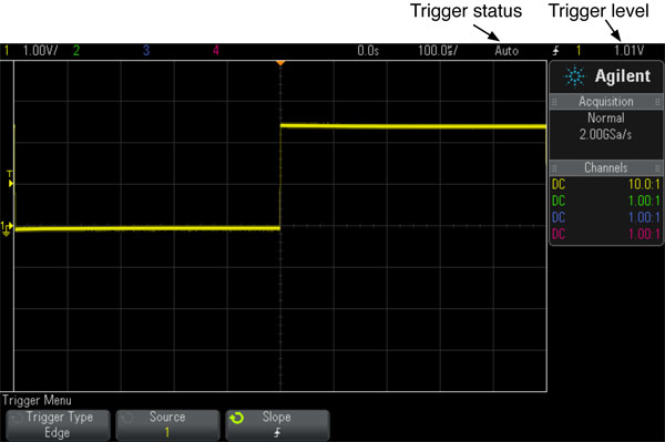
The trigger level is always indicated on the display with the small "T" and triangle along the left side of the display. When the level is being adjusted it also shows it as a horizontal line through the display. Look at the top center part of the display and there should be small solid triangle pointing down. This indicator shows the point along the horizontal (time) axis where the trigger condition was met. The default position is in the middle of the screen so you can see what the signal looked like before and after the triggering occurred.

7. We can change the horizontal position on the screen of the triggering point. In the Horizontal section of the front panel (see below), try rotating the small knob on the right. This is the Horizontal Postion control and the little solid triangle (and the displayed signal) will move right or left on the screen showing more of the signal before or after the trigger point. This can be very useful if you want to see what happened with a signal some time before or after the point where the scope was triggered.

   

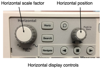
   Useful Tip: If the trigger point has been moved left or right so much that it's not visible on the screen, this is indicated with an empty triangle at the top of the display. You can always return the trigger point to the center of the screen by pressing the horizontal position knob.

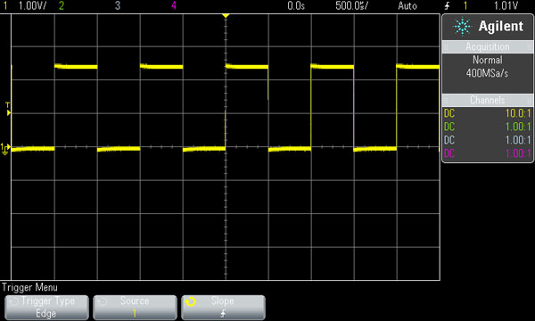
8. The last step is to change the horizontal scale factor, also known as the "time base" so we can see more of what the signal looks like. Rotate the large knob in the Horizontal section of the front panel to change the time per division (shown at the top of the display) until it says 500μs. We can now see that the signal is a square wave that repeats every 1000 microseconds, or 1msec. From the vertical scale we can see that the signal goes between zero volts and +2.5 volts.

   

9. Try playing with the controls (horizontal scale, vertical scale, horizontal position, vertical position, trigger level) to get a feel for how they affect what you see on the screen. Note that using the vertical position control to move the trace up and down on the screen does not affect the triggering level, it moves with the trace.

 

Part 2: Observing Arduino Outputs

In following lab tasks you will use your Arduino to generate a number of signals, and make measurements of these signals using the oscilloscope.

Setup

The Arduino Uno is a microcomputer development board based on an Atmel ATmega328P eight-bit microcontroller. Along with the microcontroller the board has connectors to allow solderless connection to the ATmega328P input and output pins, a clock oscillator, a second microcontroller for implementing a USB interface, and other related components. As can be seen below, the Uno has 13 I/O ports along the top that are labeled "Digital (PWM-)". These are referred to as ports D0 through D13 in the notes below. The six I/O ports at the lower right are labeled "Analog In" on the board and these are referred to as ports A0 through A5 below.

There are also a few places on these connectors where you can make connections to the ground on the Arduino. In all our Arduino lab exercises we will need to use one of these to make sure the Arduino's ground is connected to the ground on our breadboard or other devices.

In this part of the lab exercise you will be downloading to the Arduino a test program that generates various signals on the Arduino's output pins. The oscilloscope will then be used to observe these signals and make measurements of them.

In your ee109 folder, create a lab2 folder.

cd Desktop
cd ee109
mkdir lab2

From the class web site download into the lab2 folder the file "lab2.zip" and extract the contents. You should end up with four files:

lab2.o

A binary file containing the program you will download to your Arduino.

uscid.c

A C file you will use to customize the program in the Arduino.

Makefile

A Makefile for use with the lab2.o and uscid.c files.

Lab2_Answers.txt

A text file that you can edit with your text editor to record your answers to the questions below. This file must be uploaded to Vocareum by the lab due date.

Now that we have the necessary Arduino files in the lab2 folder, we need to build the Arduino program that will generate the signals.

1. Open the uscid.c file with your text editor. It only has a couple of lines and should look like this.

   #define USCID 1234567890
   
   unsigned long long hash = USCID;
   

2. Use your text editor to change the 10 digit number on the first line to be your USCid number (without any dashes), and then save and close the file. Note: If you are working with partner for this lab, just pick one of the partners USCid number and use that one. You don't have to repeat the following measurements for each person in the group.
3. Plug the USB cable into a port on your computer and then plug it into the USB connector on the Arduino board.
4. As was done in Lab 0 a couple weeks ago, you may have to use the text editor to change the PROGRAMMER line at the top of the Makefile to make it work on your computer.

Useful tip: In Lab 1 we compiled the program with the command "make" and then downloaded it with the command "make flash". If instead you just type "make flash", the program will check to see if the program needs to be compiled before downloading it. If so, it will do the compile steps as if you had typed "make", and then it will do the downloading. Only having to type "make flash" each time you want to reprogram the Arduino can speed things up, but also makes it difficult to see if the compiling generated any warnings.

5. Type the command "make flash". This will build the Lab 2 test program and download the program data to the Uno.
6. If the test program has been successfully downloaded to the Arduino the LED near the D13 I/O pin should start to blink a heartbeat pattern about once each second.

The program in the Arduino is now generating a number of signals on the output pins and we want to observe these signals with the oscilloscope. The microcontroller input and outputs pins are all connected to one of the four black connectors along the edges of the boards. To connect the scope probes to one of these signals,

• Take a short (1-2 inch) piece of wire and strip about 1/4" off each end.
• Insert one end down into the hole in the black connector for the signal you wish to measure.
• Hook the probe clip to the other end of the wire.
• Do the same for the scope probe's black ground connector so the Arduino's ground and the scope's ground are connected together. The wire from the probe's ground clip should be inserted into one of the ground connections on the board (labeled "GND").

An example of this is shown in below, however you will be plugging wires into different holes on the connectors than is shown below.

Task 1: Measure Periodic Signals

Output ports A0 and A1 are generating two periodic signals oscillating at two different frequencies. These are digital signals that transition very rapidly between the two logic states: 0 and 1. When the signal is low (very close to the "Ground" level) it is in the 0 state. When the signal is high, probably about +5V in this case, it is in the 1 state.

Connect the oscilloscope probe to port A0 and adjust the display and trigger settings to get a stable display on the screen where you can analyze the timing of the signal. The following measurements need to be made:

Time in the 1 state

Use the horizontal scale factor and the grid lines on the screen to determine this. For example if a signal is high for 2.6 divisions and the horizontal scale is set to 200μs per division, then the signal is high for 2.6 × 200μs = 520 μs. Remember to specify the units of time: ms, μs or ns.

Time in the 0 state

Same as above but measure when the signal is low.

Period

This is the time it take for a periodic signal to repeat. It should be the sum of the time in the 1 state plus the time in the 0 state.

Frequency

The frequency of he signal is the inverse of the period. For example, if the period is 2ms, then the frequency is given by

Duty cycle

The duty cycle of a signal is the ratio (expressed as a percentage) of the time the signal is in the 1 state (high) to the period of the signal.

Once you have made these measurements for the A0 output, repeat the analysis for the A1 output. The two signals should be oscillating at different frequencies.

Question 1:

Enter the results of your measurements for the A0 and A1 signals in the Lab2_Answers.txt file.

Checkpoint: Show a CP your measurements of the two periodic signals to received the bonus points.

Task 2: Measuring Non-Periodic Signals

For this task you will configure the scope to watch for a non-repeating event, one that only happens occasionally, as opposed to the repetitive periodic signals we have observed earlier in this lab. Being able to look at signals that only change occasionally can be very useful when debugging a digital system.

The signal on output port A2 is not periodic. It is in the low state most of the time but occasionally goes high for a short time. This type of signal is called a "pulse". This pulse appears at random times and the pulse width, the time it is in the high state, varies slightly each time. To see signals like this the scope has to take a single acquisition of the signal and then hold it so it can be viewed.

Connect the oscilloscope probe to port A2 and adjust the scope triggering settings as described below.

1. Trigger on a rising edge ("Slope" set for signal going from low to high)
2. Trigger channel set to whichever scope channel is connected to A2
3. Triggering level set to about 2.5 volts.

To capture a pulse, press the "Single" button in the upper right. This tells the scope to wait for the next time the input matches the trigger condition, capture and display the signal, and then freeze the display so we can look at it. It's like taking a digital photo of the signal. The pulse appears on the A2 pin at random times so it may take a few seconds before one occurs. Once the scope acquires the signal it will display it on the screen.

You may have to make several acquisitions of the A2 signal with different settings of the horizontal rate setting, and if necessary the horizontal position, to expand the pulse and position it where you can see its shape and measure the width of the pulse.

Once you have the settings correct to show the shape and size of the signal, repeat the pulse capture about 10 times and determine the approximate range (in ms, μs or ns) of the pulse width.

Question 2:

What is the minimum and maximum width of the A2 pulse that you observed?

Part 3: Observing Signal Transitions

In this section we want to look at both the input and output of a digital circuit so we can determine how the output was caused by the input. For example, in the circuit you built in Lab 1 when the button is pressed the output will change and we want to be able to use the scope to observe the nature of the input and output signals at the instant the signals changes.

To observe these signals start with the following steps.

1. We will use the circuit from Lab 1 that used a button to turn an LED on and off (shown below). If you disassembled that circuit you will have to rebuild it on the breadboard before proceeding.
2. Get a second probe from the scope's storage compartment. Attach the probe with the yellow band to channel 1, and the one with the green band to channel 2.
3. Turn on channel 2 by pressing the button with the big "2" on it above the position knob for channel 2. This should put a green signal trace somewhere on the screen.
4. Adjust the vertical scale for both channels to be 2.0V per division.
5. Use the positioning controls to put the yellow trace three divisions below the top of the screen, and put the green trace one division above the bottom.
6. Adjust the horizontal scale setting to 100ns per division.
7. Set the triggering for edge triggering, channel 1 and falling edge. We have to set it to a falling edge since we want to trigger when the button pressed, and when that happens the button signal goes from 1 to 0.
8. Use the Level knob to set the trigger voltage to 2.0 Volts. This is about midway between the voltage for a logical 1 and a logical 0.
9. Press the horizontal position knob near the top of the controls to move the trigger point to the middle of the screen.

The next step is to connect the scope to both the input signal and the output signal so both can be observed together. We are going to use channel 1 to observe the input signal and channel 2 to see the output signal.

10. Attach the probe for channel 1 to the circuit node where the button, its pull-up resistor and the inverter are connected as shown below.
11. Attach the probe for channel 2 to the output of the inverter.
12. Attach one or both of the two probe ground wires to the breadboard ground.

With the button not pressed the input signal is a logical 1 and you should see the channel 1 yellow trace at just under 5V, indicating a logical 1 state. The channel 2 green trace should be near 0V indicating a logical 0 state on the inverter output.

Press the button to make the input go to a logical 0 state. Both traces should move, the yellow from around 5V down to 0V, and the green from 0V up to near 5V. This shows the inverter circuit is working but about all we can see is two horizontal lines moving up and down as the button is pressed and released. The signals change too quickly to see the point where they make a transition from a logical 0 to a logical 1 or vice-versa. To see that we have to capture the signals at the instant they change and freeze the display.

Press the "Single" button in the upper right. Both traces will disappear from the screen since the scope is waiting for that trigger condition to occur. Now try pressing the button to change the input. The scope should acquire the signals as they are changing and display them frozen on the screen as shown in the picture below.

From the scope display we can see the input (yellow trace) made a transition from 1 to 0 when the button was pressed, and the inverter output (green trace) responded by going from 0 to 1. you may also be able to see a small propagation delay from the input to the output since the output signal (green) is lagging behind the input signal (yellow).

Task 3: Measure the propagation delay

The picture above shows the signals moving (input goes down, output goes up) but we can't really see how long the delay is from input to output. We need use the horizontal timing control to effectively zoom in on the point where the signals changes. Use the horizontal timing control to speed up the drawing of the signals from 100ns per division to something faster (less time per division). Try several different faster times and each time a change has been made, repeat the acquisition of the signals until you get a better view of the delay.

You should be able to see from the display that the signals don't change instantly, they "ramp" up from low voltage (logic 0) to high voltage (logic 1) or vice versa. In order to determine the propagation delay we have to decide what voltage do we consider to be the point where the signal has changed from 0 to 1 or 1 to 0. For your measurements here, use 2.0 volts as the logic threshold. We want to use the scope to determine how long from when the input signal crossed 2.0 volts as it went down from 5V to 0V until the output signal crossed 2.0V as it went up from 0V to 5V (or whatever level it rose to.)

To do this first use the Vertical Position controls to put the ground levels for both traces on two different horizontal grid lines as shown in picture above. Then use the Horizontal Position control to move the signals sideways to put the point where the input signal as it goes down reaches 2.0V on one of the vertical grid lines. Then observe how many horizontal grid divisions there are until the output signal reaches 2.0V as it goes up, and from that calculate the time for the propagation delay.

Question 3:

What is the approximate time delay from input to output of the NOT gate? Remember to show the units.

Part 4: Logic Thresholds

Logic circuits have to interpret voltage levels and determine if the voltage represents a logical zero or one. This usually down by setting a threshold voltage in logic circuit. If the input voltage is below the threshold, it's interpreted as a logical zero, and if it's above the threshold it's considered to be a one. In the previous task we measured the propagation delay through a NOT gate by assuming an arbitrary logic threshold of 2.0V. In this task we will try to determine what the actual threshold voltage is for the 74HCT04 inverter.

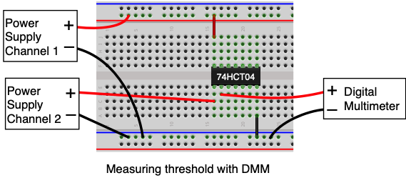
In this experiment channel 1 will provide power to the IC and channel 2 will serve as the input signal. Note on the diagram below that all four black wires from the 74HCT04, both power supplies and DMM plug into ground bus. This connects them all together and establishes a common ground for both power supplies, the DMM and the 74HCT04.

Task 4: Measure the logic threshold

1. Turn off the outputs of the power supply.
2. You can start with your breadboard circuit from Part 3 above that used a 74HCT04 and turned an LED on and off with a button. If you haven't done so already, remove the LED, the switch and the two resistors from the board. All you need on the breadboard for this experiment is the 74HCT04 and its power and ground wires.
3. Set channel 1 of the power supply to output +5V. Connect the black lead from channel 1 to the ground bus on the breadboard and connect the red lead to the red power bus.
4. Set the DMM to display DC volts and connect the read lead to inverter output (pin 2) of the IC. The black lead from the DMM should be connected to the ground bus on the breadboard.
5. As you did for channel 1 at the start of Lab 1, now set the current limit for channel 2 of the power supply to something like 0.3A.
6. Set the output voltage of channel 2 of the power supply to 0V. Connect the black lead from channel 2 to the ground bus and connect the red lead to inverter input (pin 1) of the 74HCT04.
7. Turn on the outputs of the power supply

Note: Once you apply power to the 74HCT04, the indicated voltage for channel 2 on the power supply may not be at 0V any longer. Even though you set it for 0V in step 5 above, the 74HCT04's input may drag the voltage up a bit when it is turned on. You can ignore this in the steps below. Just record the value you set the power supply to even though it may show a different value on the display.

The DMM should show a voltage of between 4 and 5 volts. Since you are putting a logical 0 on the input of the inverter, the output is in the logical one state which for this type of IC is a voltage above 4 volts.

Select channel 2 on the power supply and move the underline cursor until it is under the tenths of a volt digit. Rotate the knob to increase the input voltage by 0.1 volts with each click of the knob and observe the inverter output voltage displayed on the DMM. Note that as you increase the input voltage the output changes very little until the input reaches the logic threshold, and then the output drops rapidly towards zero volts.

Question 4:

Show the measured output voltages for the input voltages listed in the table on the question sheet.

Results

The answers to the above questions should be edited into the "Lab2_Answers.txt" file and the file uploaded to the Vocareum web site by the due date. See the Assignments page of the class web site for a link for uploading.

Review Questions

Answer the following questions in your "Lab2_Answers.txt".

1. Suppose you wanted to measure the frequency of a note played by a piano and sensed from a microphone connected/viewed on an oscilloscope. Answer the following True/False questions with a brief explanation.

   1. T/F: To measure the frequency, the vertical scale of the oscilloscope would be of more use than the horizontal scale.
   2. T/F: Since the note is played for a short time period, we should set the triggering to "Single" rather than "Run".
   3. T/F: If the signal ranges between 0V and 2.5V, the trigger level should ideally be set around 1.25V.
2. Each scope probe has a short black ground wire attached to it. Why is it necessary to connect this to the circuit's ground point in order to make a measurement?
3. If you have used the Horizontal Position control to move the trigger point horizontally so much that you can no longer see the trigger point on the screen, what is the quick way to restore the trigger point back to the middle of the screen?